bayesDP/��������������������������������������������������������������������������������������������0000755�0001777�0001777�00000000000�13145350215�013132� 5����������������������������������������������������������������������������������������������������ustar �herbrandt�����������������������herbrandt��������������������������������������������������������������������������������������������������������������������������������������������������������������������������������������������������������������bayesDP/inst/���������������������������������������������������������������������������������������0000755�0001777�0001777�00000000000�13144711751�014114� 5����������������������������������������������������������������������������������������������������ustar �herbrandt�����������������������herbrandt��������������������������������������������������������������������������������������������������������������������������������������������������������������������������������������������������������������bayesDP/inst/doc/�����������������������������������������������������������������������������������0000755�0001777�0001777�00000000000�13144711751�014661� 5����������������������������������������������������������������������������������������������������ustar �herbrandt�����������������������herbrandt��������������������������������������������������������������������������������������������������������������������������������������������������������������������������������������������������������������bayesDP/inst/doc/bdpnormal-vignette.html������������������������������������������������������������0000644�0001777�0001777�00000523327�13144711745�021367� 0����������������������������������������������������������������������������������������������������ustar �herbrandt�����������������������herbrandt��������������������������������������������������������������������������������������������������������������������������������������������������������������������������������������������������������������
Introduction
Introduction
The purpose of this vignette is to introduce the bdpnormal function. bdpnormal is used for estimating posterior samples from a Gaussian mean outcome for clinical trials where an informative prior is used. In the parlance of clinical trials, the informative prior is derived from historical data. The weight given to the historical data is determined using what we refer to as a discount function. There are three steps in carrying out estimation:
Estimation of the historical data weight, denoted \(\hat{\alpha}\), via the discount function
Estimation of the posterior distribution of the current data, conditional on the historical data weighted by \(\hat{\alpha}\)
If a two-arm clinical trial, estimation of the posterior treatment effect, i.e., treatment versus control
Throughout this vignette, we use the terms current, historical, treatment, and control. These terms are used because the model was envisioned in the context of clinical trials where historical data may be present. Because of this terminology, there are 4 potential sources of data:
Current treatment data: treatment data from a current study
Current control data: control (or other treatment) data from a current study
Historical treatment data: treatment data from a previous study
Historical control data: control (or other treatment) data from a previous study
If only treatment data is input, the function considers the analysis a one-arm trial. If treatment data + control data is input, then it is considered a two-arm trial.
Estimation of the historical data weight
In the first estimation step, the historical data weight \(\hat{\alpha}\) is estimated. In the case of a two-arm trial, where both treatment and control data are available, an \(\hat{\alpha}\) value is estimated separately for each of the treatment and control arms. Of course, historical treatment or historical control data must be present, otherwise \(\hat{\alpha}\) is not estimated for the corresponding arm.
When historical data are available, estimation of \(\hat{\alpha}\) is carried out as follows. Let \(\bar{y}\), \(s\), and \(N\) denote the sample mean, sample standard deviation, and sample size of the current data, respectively. Similarly, let \(\bar{y}_0\), \(s_0\), and \(N_0\) denote the sample mean, sample standard deviation, and sample size of the historical data, respectively. Then, the posterior distribution of the mean for current data, under vague (flat) priors is
\[ \begin{array}{rcl}
\tilde{\sigma}^2\mid\bar{y},s,N & \sim & InverseGamma\left(\frac{N-1}{2},\,\frac{N-1}{2}s^2 \right),\
\
\tilde{\mu}\mid\bar{y},N,\tilde{\sigma}^2 & \sim & \mathcal{N}ormal\left(\bar{y},\, \frac{1}{N}\tilde{\sigma}^2 \right).
\end{array}
\]
Similarly, the posterior distribution of the mean for historical data, under vague (flat) priors is
\[ \begin{array}{rcl}
\sigma^2_0 & \sim & InverseGamma\left(\frac{N_0-1}{2},\,\frac{N_0-1}{2}s_0^2 \right),\
\
\mu_0 \mid \bar{y}_0, N_0, \sigma^2_0 & \sim & \mathcal{N}ormal\left(\bar{y}_0,\, \frac{1}{N_0}\sigma^2_0 \right).
\end{array}
\]
We next compute the posterior probability \(p = Pr\left(\tilde{\mu} < \mu_0\mid\bar{y},s,N,\bar{y}_0,s_0,N_0\right)\). Finally, for a Weibull distribution function (i.e., the Weibull cumulative distribution function), denoted \(W\), \(\hat{\alpha}\) is computed as
\[
\begin{array}{ccc}
\mbox{One-sided analysis} & & \mbox{Two-sided analysis} \
\hat{\alpha}=\alpha_{max}\cdot W\left(p, \,w_{shape}, \,w_{scale}\right),
& &
\hat{\alpha}=\begin{cases}
\alpha_{max}\cdot W\left(p, \,w_{shape}, \,w_{scale}\right),\,0\le p\le0.5\
\alpha_{max}\cdot W\left(1-p, \,w_{shape}, \,w_{scale}\right),\,0.5 \lt p \le 1,
\end{cases}
\end{array}
\]
where \(w_{shape}\) and \(w_{scale}\) are the shape and scale of the Weibull distribution function, respectively and \(\alpha_{max}\) scales the weight \(\hat{\alpha}\) by a user-input maximum value. Using the default values of \(w_{shape}=3\) and \(w_{scale}=0.135\), \(\hat{\alpha}\) increases to 1 as \(p\) increases to 1 (one-sided) and \(\hat{\alpha}\) increases to 1 as \(p\) goes to 0.5 (two-sided).
There are several model inputs at this first stage. First, the user can select fix_alpha=TRUE and force a fixed value of \(\hat{\alpha}\) (at the alpha_max input), as opposed to estimation via the discount function. Next, a Monte Carlo estimation approach is used, requiring several samples from the posterior distributions. Thus, the user can input a sample size greater than or less than the default value of number_mcmc=10000. Finally, the shape of the Weibull discount function can be altered by changing the Weibull shape and scale parameters from the default values of \(w_{shape}=3\) and \(w_{scale}=0.135\) (weibull_shape and weibull_scale inputs).
An alternate Monte Carlo-based estimation scheme of \(\hat{\alpha}\) has been implemented, controlled by the function input method="mc". Here, instead of treating \(\hat{\alpha}\) as a fixed quantity, \(\hat{\alpha}\) is treated as random. First, \(p\), is computed as
\[ \begin{array}{rcl}
Z & = & \displaystyle{\frac{\left(\mu-\mu_0\right)^2}{\sigma^2 + \sigma^2_0}} ,\
\
p & = & \chi^2_{Z,1},
\end{array}
\]
where \(\chi^2_{x,d}\) is the $x$th quantile of a chi-square distribution with \(d\) degrees of freedom (the value \(p\) is found via the pchisq R function using lower.tail=FALSE). Next, \(p\) is used to construct \(\hat{\alpha}\) using the one-sided analysis approach described above. Since the values \(Z\) and \(p\) are computed at each iteration of the Monte Carlo estimation scheme, \(\hat{\alpha}\) is computed at each iteration of the Monte Carlo estimation scheme, resulting in a distribution of \(\hat{\alpha}\) values.
With the historical data weight (or weights) \(\hat{\alpha}\) in hand, we can move on to estimation of the posterior distribution of the current data.
Discount function
Throughout this vignette, we refer to a discount function. The discount function is a Weibull distribution function and has the form
\[W(x) = 1 - \exp\left\{- (x/w_{scale})^{w_{shape}}\right\}.\]
During estimation, a user may be interested in selecting values of \(w_{shape}\) and \(w_{scale}\) that result in optimal statistical properties of the analysis. Thus, the discount function can be used to control the false positive rate (type I error) and/or the false negative rate (type II error). Examples in a following section illustrate the shape of the discount function using the default shape and scale parameters.
Another important aspect related to the discount function is the analysis type: one-sided or two-sided. The sidedness of the analysis is analogous to a one- or two-sided hypothesis test. Using the default shape and scale inputs, a two-sided analysis type results in a discount function with the following curve:

The discount function of a one-sided analysis, again with the default shape and scale inputs, has the following curve:

In both of the above plots, the x-axis is the stochastic comparison between current and historical data, which we've denoted \(p\). The y-axis is the discount value \(\hat{\alpha}\) that corresponds to a given value of \(p\).
An advanced input for the plot function is print. The default value is print = TRUE, which simpy returns the graphics. Alternately, users can specify print = FALSE, which returns a ggplot2 object. Below is an example using the discount function plot:
p1 <- plot(fit01, type="discount", print=FALSE)
p1 + ggtitle("Discount Function Plot :-)")

Estimation of the posterior distribution of the current data, conditional on the historical data
With \(\hat{\alpha}\) in hand, we can now estimate the posterior distribution of the mean of the current data. Using the notation of the previous section, the posterior distribution is
\[\mu \sim \mathcal{N}ormal\left( \frac{\sigma^2_0N\bar{y} + \tilde{\sigma}^2N_0\bar{y}_0\hat{\alpha}}{N\sigma^2_0 + \tilde{\sigma}^2N_0\hat{\alpha}},\,\frac{\tilde{\sigma}^2\sigma^2_0}{N\sigma^2_0 + \tilde{\sigma}^2N_0\hat{\alpha}} \right).\]
At this model stage, we have in hand number_mcmc simulations from the augmented mean distribution. If there are no control data, i.e., a one-arm trial, then the modeling stops and we generate summaries of the posterior distribution of \(\mu\). Otherwise, if there are control data, we proceed to a third step and compute a comparison between treatment and control data.
Estimation of the posterior treatment effect: treatment versus control
This step of the model is carried out on-the-fly using the summary or print methods. Let \(\mu_T\) and \(\mu_C\) denote posterior mean estimates of the treatment and control arms, respectively. Currently, the implemented comparison between treatment and control is the difference, i.e., summary statistics related to the posterior difference: \(\mu_T - \mu_C\). In a future release, we may consider implementing additional comparison types.
Function inputs
The data inputs for bdpnormal are mu_t, sigma_t, N_t, mu0_t, sigma0_t, N0_t, mu_c, sigma_c, N_c, mu0_c, sigma0_c, and N0_c. The data must be input as (mu, sigma, N) triplets For example, mu_t, the sample mean of the current treatment group, must be accompanied by sigma_t and N_t, the sample standard deviation and sample size, respectively. Historical data inputs are not necessary, but using this function would not be necessary either.
At the minimum, mu_t, sigma_t, and N_t must be input. In the case that only mu_t, sigma_t, and N_t are input, the analysis is analogous to a one-sample t-test.. Each of the following input combinations are allowed:
- (
mu_t, sigma_t, N_t) - one-arm trial
- (
mu_t, sigma_t, N_t) + (mu0_t, sigma0_t, N0_t) - one-arm trial
- (
mu_t, sigma_t, N_t) + (mu_c, sigma_c, N_c) - two-arm trial
- (
mu_t, sigma_t, N_t) + (mu0_c, sigma0_c, N0_c) - two-arm trial
- (
mu_t, sigma_t, N_t) + (mu0_t, sigma0_t, N0_t) + (mu_c, sigma_c, N_c) - two-arm trial
- (
mu_t, sigma_t, N_t) + (mu0_t, sigma0_t, N0_t) + (mu0_c, sigma0_c, N0_c) - two-arm trial
- (
mu_t, sigma_t, N_t) + (mu0_t, sigma0_t, N0_t) + (mu_c, sigma_c, N_c) + (mu0_c, sigma0_c, N0_c) - two-arm trial
Examples
One-arm trial
Suppose we have historical data with a mean of mu0_t=50, standard deviation of sigma0_t=5, and sample size of N0_t=250 patients. Also suppose that we have current data with a mean of mu_t=30, standard deviation of sigma_t=10, and sample size of N_t=250. To illustrate the approach, let's first give full weight to the historical data. This is accomplished by setting alpha_max=1 and fix_alpha=TRUE as follows:
set.seed(42)
fit1 <- bdpnormal(mu_t = 30,
sigma_t = 10,
N_t = 250,
mu0_t = 50,
sigma0_t = 5,
N0_t = 250,
alpha_max = 1,
fix_alpha = TRUE)
summary(fit1)
##
## One-armed bdp normal
##
## data:
## Current treatment: mu_t = 30, sigma_t = 10, N_t = 250
## Historical treatment: mu0_t = 50, sigma0_t = 5, N0_t = 250
## Stochastic comparison (p_hat) - treatment (current vs. historical data): 1
## Discount function value (alpha) - treatment: 1
## 95 percent confidence interval:
## 44.985 46.922
## augmented sample estimate:
## mean of treatment group
## 45.9982
Based on the summary output of fit1, we can see that the value of alpha was held fixed at 1. The resulting (augmented) mean was estimated at 45.9982. Note that the print and summary methods result in the same output.
Now, let's relax the constraint on fixing alpha at 1. We'll also take this opportunity to describe the output of the plot method.
set.seed(42)
fit1a <- bdpnormal(mu_t = 30,
sigma_t = 10,
N_t = 250,
mu0_t = 50,
sigma0_t = 5,
N0_t = 250,
fix_alpha = FALSE)
summary(fit1a)
##
## One-armed bdp normal
##
## data:
## Current treatment: mu_t = 30, sigma_t = 10, N_t = 250
## Historical treatment: mu0_t = 50, sigma0_t = 5, N0_t = 250
## Stochastic comparison (p_hat) - treatment (current vs. historical data): 0
## Discount function value (alpha) - treatment: 0
## 95 percent confidence interval:
## 28.74 31.2272
## augmented sample estimate:
## mean of treatment group
## 29.9963
When alpha is not constrained to one, it is estimated based on a comparison between the current and historical data. We see that the stochastic comparison, p_hat, between historical and control is 1. Here, p_hat is the posterior probability that the current sample mean is less than the historical sample mean under vague priors. With the present example, p_hat = 1 implies that the current and historical sample means are very different. The result is that the weight given to the historical data is shrunk towards zero. Thus, the estimate of alpha from the discount function is 0 and the augmented posterior estimate of the mean is approximately the mean of the current data.
Many of the the values presented in the summary method are accessible from the fit object. For instance, alpha is found in fit1a$posterior_treatment$alpha_discount and p_hat is located at fit1a$posterior_treatment$p_hat. The augmented mean and confidence interval are computed at run-time. The results can be replicated as:
mean_augmented <- round(median(fit1a$posterior_treatment$posterior_mu),4)
CI95_augmented <- round(quantile(fit1a$posterior_treatment$posterior_mu, prob=c(0.025, 0.975)),4)
Finally, we'll explore the plot method.
plot(fit1a)


The top plot displays three density curves. The blue curve is the density of the historical mean, the green curve is the density of the current mean, and the red curve is the density of the current mean augmented by historical data. Since little weight was given to the historical data, the current and posterior means essentially overlap.
The middle plot simply re-displays the posterior mean.
The bottom plot displays the discount function (solid curve) as well as alpha (horizontal dashed line) and p_hat (vertical dashed line). In the present example, the discount function is the Weibull probability distribution with shape=3 and scale=0.135.
Two-arm trial
On to two-arm trials. In this package, we define a two-arm trial as an analysis where a current and/or historical control arm is present. Suppose we have the same treatment data as in the one-arm example, but now we introduce control data: mu_c = 25, sigma_c = 10, N_c = 250, mu0_c = 25, sigma0_c = 5, and N0_c = 250.
Before proceeding, it is worth pointing out that the discount function is applied separately to the treatment and control data. Now, let's carry out the two-arm analysis using default inputs:
set.seed(42)
fit2 <- bdpnormal(mu_t = 30,
sigma_t = 10,
N_t = 250,
mu0_t = 50,
sigma0_t = 5,
N0_t = 250,
mu_c = 25,
sigma_c = 10,
N_c = 250,
mu0_c = 25,
sigma0_c = 5,
N0_c = 250,
fix_alpha = FALSE)
summary(fit2)
##
## Two-armed bdp normal
##
## data:
## Current treatment: mu_t = 30, sigma_t = 10, N_t = 250
## Current control: mu_c = 25, sigma_c = 10, N_c = 250
## Historical treatment: mu0_t = 50, sigma0_t = 5, N0_t = 250
## Historical control: mu0_c = 25, sigma0_c = 5, N0_c = 250
## Stochastic comparison (p_hat) - treatment (current vs. historical data): 0
## Stochastic comparison (p_hat) - control (current vs. historical data): 0.4935
## Discount function value (alpha) - treatment: 0
## Discount function value (alpha) - control: 1
## alternative hypothesis: two.sided
## 95 percent confidence interval:
## 3.6263 6.3496
## augmented sample estimates:
## treatment group control group
## 30.00 25.00
The summary method of a two-arm analysis is slightly different than a one-arm analysis. First, we see p_hat and alpha reported for the control data. In the present analysis, the current and historical control data have sample means that are very close, thus the historical control data is given full weight. Again, little weight is given to the historical treatment data.
The confidence interval is computed at run time and is the interval estimate of the difference between the posterior means of the treatment and control groups. With a 95% confidence interval of (3.6263, 6.3496), we would conclude that the treatment and control arms are not significantly different.
The plot method of a two-arm analysis is slightly different than a one-arm analysis as well:
plot(fit2)


 Each of the three plots are analogous to the one-arm analysis, but each plot now presents additional data related to the control arm.
���������������������������������������������������������������������������������������������������������������������������������������������������������������������������������������������������������������������������������������������������������������������������������������������������������bayesDP/inst/doc/bdpnormal-vignette.Rmd�������������������������������������������������������������0000644�0001777�0001777�00000040463�13127717076�021144� 0����������������������������������������������������������������������������������������������������ustar �herbrandt�����������������������herbrandt��������������������������������������������������������������������������������������������������������������������������������������������������������������������������������������������������������������---
title: "BayesDP"
author: "Donnie Musgrove"
date: "`r Sys.Date()`"
output:
rmarkdown::html_vignette:
toc: yes
fig_caption: yes
params:
# EVAL: !r identical(Sys.getenv("NOT_CRAN"), "true")
# EVAL: !r FALSE
vignette: >
%\VignetteIndexEntry{Normal Mean Estimation}
%\VignetteEngine{knitr::rmarkdown}
%\VignetteEncoding{UTF-8}
---
```{r, SETTINGS-knitr, include=FALSE}
library(bayesDP)
stopifnot(require(knitr))
opts_chunk$set(
#comment = NA,
#message = FALSE,
#warning = FALSE,
#eval = if (isTRUE(exists("params"))) params$EVAL else FALSE,
dev = "png",
dpi = 150,
fig.asp = 0.8,
fig.width = 5,
out.width = "60%",
fig.align = "center"
)
# Run two models to document the discount function plots
fit01 <- bdpnormal(mu_t=10, sigma_t = 1, N_t=500,
mu0_t=10, sigma0_t = 1, N0_t=500, two_side=FALSE)
fit02 <- bdpnormal(mu_t=10, sigma_t = 1, N_t=500,
mu0_t=10, sigma0_t = 1, N0_t=500)
```
# Introduction
The purpose of this vignette is to introduce the `bdpnormal` function. `bdpnormal` is used for estimating posterior samples from a Gaussian mean outcome for clinical trials where an informative prior is used. In the parlance of clinical trials, the informative prior is derived from historical data. The weight given to the historical data is determined using what we refer to as a discount function. There are three steps in carrying out estimation:
1. Estimation of the historical data weight, denoted $\hat{\alpha}$, via the discount function
2. Estimation of the posterior distribution of the current data, conditional on the historical data weighted by $\hat{\alpha}$
3. If a two-arm clinical trial, estimation of the posterior treatment effect, i.e., treatment versus control
Throughout this vignette, we use the terms `current`, `historical`, `treatment`, and `control`. These terms are used because the model was envisioned in the context of clinical trials where historical data may be present. Because of this terminology, there are 4 potential sources of data:
1. Current treatment data: treatment data from a current study
2. Current control data: control (or other treatment) data from a current study
3. Historical treatment data: treatment data from a previous study
4. Historical control data: control (or other treatment) data from a previous study
If only treatment data is input, the function considers the analysis a one-arm trial. If treatment data + control data is input, then it is considered a two-arm trial.
## Estimation of the historical data weight
In the first estimation step, the historical data weight $\hat{\alpha}$ is estimated. In the case of a two-arm trial, where both treatment and control data are available, an $\hat{\alpha}$ value is estimated separately for each of the treatment and control arms. Of course, historical treatment or historical control data must be present, otherwise $\hat{\alpha}$ is not estimated for the corresponding arm.
When historical data are available, estimation of $\hat{\alpha}$ is carried out as follows. Let $\bar{y}$, $s$, and $N$ denote the sample mean, sample standard deviation, and sample size of the current data, respectively. Similarly, let $\bar{y}_0$, $s_0$, and $N_0$ denote the sample mean, sample standard deviation, and sample size of the historical data, respectively. Then, the posterior distribution of the mean for current data, under vague (flat) priors is
$$ \begin{array}{rcl}
\tilde{\sigma}^2\mid\bar{y},s,N & \sim & InverseGamma\left(\frac{N-1}{2},\,\frac{N-1}{2}s^2 \right),\\
\\
\tilde{\mu}\mid\bar{y},N,\tilde{\sigma}^2 & \sim & \mathcal{N}ormal\left(\bar{y},\, \frac{1}{N}\tilde{\sigma}^2 \right).
\end{array}
$$
Similarly, the posterior distribution of the mean for historical data, under vague (flat) priors is
$$ \begin{array}{rcl}
\sigma^2_0 & \sim & InverseGamma\left(\frac{N_0-1}{2},\,\frac{N_0-1}{2}s_0^2 \right),\\
\\
\mu_0 \mid \bar{y}_0, N_0, \sigma^2_0 & \sim & \mathcal{N}ormal\left(\bar{y}_0,\, \frac{1}{N_0}\sigma^2_0 \right).
\end{array}
$$
We next compute the posterior probability $p = Pr\left(\tilde{\mu} < \mu_0\mid\bar{y},s,N,\bar{y}_0,s_0,N_0\right)$. Finally, for a Weibull distribution function (i.e., the Weibull cumulative distribution function), denoted $W$, $\hat{\alpha}$ is computed as
$$
\begin{array}{ccc}
\mbox{One-sided analysis} & & \mbox{Two-sided analysis} \\
\hat{\alpha}=\alpha_{max}\cdot W\left(p, \,w_{shape}, \,w_{scale}\right),
& &
\hat{\alpha}=\begin{cases}
\alpha_{max}\cdot W\left(p, \,w_{shape}, \,w_{scale}\right),\,0\le p\le0.5\\
\alpha_{max}\cdot W\left(1-p, \,w_{shape}, \,w_{scale}\right),\,0.5 \lt p \le 1,
\end{cases}
\end{array}
$$
where $w_{shape}$ and $w_{scale}$ are the shape and scale of the Weibull distribution function, respectively and $\alpha_{max}$ scales the weight $\hat{\alpha}$ by a user-input maximum value. Using the default values of $w_{shape}=3$ and $w_{scale}=0.135$, $\hat{\alpha}$ increases to 1 as $p$ increases to 1 (one-sided) and $\hat{\alpha}$ increases to 1 as $p$ goes to 0.5 (two-sided).
There are several model inputs at this first stage. First, the user can select `fix_alpha=TRUE` and force a fixed value of $\hat{\alpha}$ (at the `alpha_max` input), as opposed to estimation via the discount function. Next, a Monte Carlo estimation approach is used, requiring several samples from the posterior distributions. Thus, the user can input a sample size greater than or less than the default value of `number_mcmc=10000`. Finally, the shape of the Weibull discount function can be altered by changing the Weibull shape and scale parameters from the default values of $w_{shape}=3$ and $w_{scale}=0.135$ (`weibull_shape` and `weibull_scale` inputs).
An alternate Monte Carlo-based estimation scheme of $\hat{\alpha}$ has been implemented, controlled by the function input `method="mc"`. Here, instead of treating $\hat{\alpha}$ as a fixed quantity, $\hat{\alpha}$ is treated as random. First, $p$, is computed as
$$ \begin{array}{rcl}
Z & = & \displaystyle{\frac{\left(\mu-\mu_0\right)^2}{\sigma^2 + \sigma^2_0}} ,\\
\\
p & = & \chi^2_{Z,1},
\end{array}
$$
where $\chi^2_{x,d}$ is the $x$th quantile of a chi-square distribution with $d$ degrees of freedom (the value $p$ is found via the `pchisq` R function using `lower.tail=FALSE`). Next, $p$ is used to construct $\hat{\alpha}$ using the one-sided analysis approach described above. Since the values $Z$ and $p$ are computed at each iteration of the Monte Carlo estimation scheme, $\hat{\alpha}$ is computed at each iteration of the Monte Carlo estimation scheme, resulting in a distribution of $\hat{\alpha}$ values.
With the historical data weight (or weights) $\hat{\alpha}$ in hand, we can move on to estimation of the posterior distribution of the current data.
### Discount function
Throughout this vignette, we refer to a discount function. The discount function is a Weibull distribution function and has the form
$$W(x) = 1 - \exp\left\{- (x/w_{scale})^{w_{shape}}\right\}.$$
During estimation, a user may be interested in selecting values of $w_{shape}$ and $w_{scale}$ that result in optimal statistical properties of the analysis. Thus, the discount function can be used to control the false positive rate (type I error) and/or the false negative rate (type II error). Examples in a following section illustrate the shape of the discount function using the default shape and scale parameters.
Another important aspect related to the discount function is the analysis type: one-sided or two-sided. The sidedness of the analysis is analogous to a one- or two-sided hypothesis test. Using the default shape and scale inputs, a __two-sided__ analysis type results in a discount function with the following curve:
```{r, echo=FALSE}
plot(fit02, type="discount")
```
The discount function of a __one-sided__ analysis, again with the default shape and scale inputs, has the following curve:
```{r, echo=FALSE}
plot(fit01, type="discount")
```
In both of the above plots, the x-axis is the stochastic comparison between current and historical data, which we've denoted $p$. The y-axis is the discount value $\hat{\alpha}$ that corresponds to a given value of $p$.
An advanced input for the plot function is `print`. The default value is `print = TRUE`, which simpy returns the graphics. Alternately, users can specify `print = FALSE`, which returns a `ggplot2` object. Below is an example using the discount function plot:
```{r}
p1 <- plot(fit01, type="discount", print=FALSE)
p1 + ggtitle("Discount Function Plot :-)")
```
## Estimation of the posterior distribution of the current data, conditional on the historical data
With $\hat{\alpha}$ in hand, we can now estimate the posterior distribution of the mean of the current data. Using the notation of the previous section, the posterior distribution is
$$\mu \sim \mathcal{N}ormal\left( \frac{\sigma^2_0N\bar{y} + \tilde{\sigma}^2N_0\bar{y}_0\hat{\alpha}}{N\sigma^2_0 + \tilde{\sigma}^2N_0\hat{\alpha}},\,\frac{\tilde{\sigma}^2\sigma^2_0}{N\sigma^2_0 + \tilde{\sigma}^2N_0\hat{\alpha}} \right).$$
At this model stage, we have in hand `number_mcmc` simulations from the augmented mean distribution. If there are no control data, i.e., a one-arm trial, then the modeling stops and we generate summaries of the posterior distribution of $\mu$. Otherwise, if there are control data, we proceed to a third step and compute a comparison between treatment and control data.
## Estimation of the posterior treatment effect: treatment versus control
This step of the model is carried out on-the-fly using the `summary` or `print` methods. Let $\mu_T$ and $\mu_C$ denote posterior mean estimates of the treatment and control arms, respectively. Currently, the implemented comparison between treatment and control is the difference, i.e., summary statistics related to the posterior difference: $\mu_T - \mu_C$. In a future release, we may consider implementing additional comparison types.
## Function inputs
The data inputs for `bdpnormal` are `mu_t`, `sigma_t`, `N_t`, `mu0_t`, `sigma0_t`, `N0_t`, `mu_c`, `sigma_c`, `N_c`, `mu0_c`, `sigma0_c`, and `N0_c`. The data must be input as (`mu`, `sigma`, `N`) triplets For example, `mu_t`, the sample mean of the current treatment group, must be accompanied by `sigma_t` and `N_t`, the sample standard deviation and sample size, respectively. Historical data inputs are not necessary, but using this function would not be necessary either.
__At the minimum, `mu_t`, `sigma_t`, and `N_t` must be input__. In the case that only `mu_t`, `sigma_t`, and `N_t` are input, the analysis is analogous to a one-sample t-test.. Each of the following input combinations are allowed:
- (`mu_t`, `sigma_t`, `N_t`) - one-arm trial
- (`mu_t`, `sigma_t`, `N_t`) + (`mu0_t`, `sigma0_t`, `N0_t`) - one-arm trial
- (`mu_t`, `sigma_t`, `N_t`) + (`mu_c`, `sigma_c`, `N_c`) - two-arm trial
- (`mu_t`, `sigma_t`, `N_t`) + (`mu0_c`, `sigma0_c`, `N0_c`) - two-arm trial
- (`mu_t`, `sigma_t`, `N_t`) + (`mu0_t`, `sigma0_t`, `N0_t`) + (`mu_c`, `sigma_c`, `N_c`) - two-arm trial
- (`mu_t`, `sigma_t`, `N_t`) + (`mu0_t`, `sigma0_t`, `N0_t`) + (`mu0_c`, `sigma0_c`, `N0_c`) - two-arm trial
- (`mu_t`, `sigma_t`, `N_t`) + (`mu0_t`, `sigma0_t`, `N0_t`) + (`mu_c`, `sigma_c`, `N_c`) + (`mu0_c`, `sigma0_c`, `N0_c`) - two-arm trial
# Examples
## One-arm trial
Suppose we have historical data with a mean of `mu0_t=50`, standard deviation of `sigma0_t=5`, and sample size of `N0_t=250` patients. Also suppose that we have current data with a mean of `mu_t=30`, standard deviation of `sigma_t=10`, and sample size of `N_t=250`. To illustrate the approach, let's first give full weight to the historical data. This is accomplished by setting `alpha_max=1` and `fix_alpha=TRUE` as follows:
```{r}
set.seed(42)
fit1 <- bdpnormal(mu_t = 30,
sigma_t = 10,
N_t = 250,
mu0_t = 50,
sigma0_t = 5,
N0_t = 250,
alpha_max = 1,
fix_alpha = TRUE)
summary(fit1)
```
Based on the `summary` output of `fit1`, we can see that the value of `alpha` was held fixed at 1. The resulting (augmented) mean was estimated at 45.9982. Note that the `print` and `summary` methods result in the same output.
Now, let's relax the constraint on fixing `alpha` at 1. We'll also take this opportunity to describe the output of the plot method.
```{r}
set.seed(42)
fit1a <- bdpnormal(mu_t = 30,
sigma_t = 10,
N_t = 250,
mu0_t = 50,
sigma0_t = 5,
N0_t = 250,
fix_alpha = FALSE)
summary(fit1a)
```
When `alpha` is not constrained to one, it is estimated based on a comparison between the current and historical data. We see that the stochastic comparison, `p_hat`, between historical and control is 1. Here, `p_hat` is the posterior probability that the current sample mean is less than the historical sample mean under vague priors. With the present example, `p_hat = 1` implies that the current and historical sample means are very different. The result is that the weight given to the historical data is shrunk towards zero. Thus, the estimate of `alpha` from the discount function is 0 and the augmented posterior estimate of the mean is approximately the mean of the current data.
Many of the the values presented in the `summary` method are accessible from the fit object. For instance, `alpha` is found in `fit1a$posterior_treatment$alpha_discount` and `p_hat` is located at `fit1a$posterior_treatment$p_hat`. The augmented mean and confidence interval are computed at run-time. The results can be replicated as:
```{r}
mean_augmented <- round(median(fit1a$posterior_treatment$posterior_mu),4)
CI95_augmented <- round(quantile(fit1a$posterior_treatment$posterior_mu, prob=c(0.025, 0.975)),4)
```
Finally, we'll explore the `plot` method.
```{r}
plot(fit1a)
```
The top plot displays three density curves. The blue curve is the density of the historical mean, the green curve is the density of the current mean, and the red curve is the density of the current mean augmented by historical data. Since little weight was given to the historical data, the current and posterior means essentially overlap.
The middle plot simply re-displays the posterior mean.
The bottom plot displays the discount function (solid curve) as well as `alpha` (horizontal dashed line) and `p_hat` (vertical dashed line). In the present example, the discount function is the Weibull probability distribution with `shape=3` and `scale=0.135`.
## Two-arm trial
On to two-arm trials. In this package, we define a two-arm trial as an analysis where a current and/or historical control arm is present. Suppose we have the same treatment data as in the one-arm example, but now we introduce control data: `mu_c = 25`, `sigma_c = 10`, `N_c = 250`, `mu0_c = 25`, `sigma0_c = 5`, and `N0_c = 250`.
Before proceeding, it is worth pointing out that the discount function is applied separately to the treatment and control data. Now, let's carry out the two-arm analysis using default inputs:
```{r}
set.seed(42)
fit2 <- bdpnormal(mu_t = 30,
sigma_t = 10,
N_t = 250,
mu0_t = 50,
sigma0_t = 5,
N0_t = 250,
mu_c = 25,
sigma_c = 10,
N_c = 250,
mu0_c = 25,
sigma0_c = 5,
N0_c = 250,
fix_alpha = FALSE)
summary(fit2)
```
The `summary` method of a two-arm analysis is slightly different than a one-arm analysis. First, we see `p_hat` and `alpha` reported for the control data. In the present analysis, the current and historical control data have sample means that are very close, thus the historical control data is given full weight. Again, little weight is given to the historical treatment data.
The confidence interval is computed at run time and is the interval estimate of the difference between the posterior means of the treatment and control groups. With a 95% confidence interval of `(3.6263, 6.3496)`, we would conclude that the treatment and control arms are not significantly different.
The `plot` method of a two-arm analysis is slightly different than a one-arm analysis as well:
```{r}
plot(fit2)
```
Each of the three plots are analogous to the one-arm analysis, but each plot now presents additional data related to the control arm.
�������������������������������������������������������������������������������������������������������������������������������������������������������������������������������������������������������������bayesDP/inst/doc/bdpsurvival-vignette.R�������������������������������������������������������������0000644�0001777�0001777�00000010675�13144711751�021201� 0����������������������������������������������������������������������������������������������������ustar �herbrandt�����������������������herbrandt��������������������������������������������������������������������������������������������������������������������������������������������������������������������������������������������������������������## ---- SETTINGS-knitr, include=FALSE--------------------------------------
library(bayesDP)
stopifnot(require(knitr))
opts_chunk$set(
#comment = NA,
#message = FALSE,
#warning = FALSE,
#eval = if (isTRUE(exists("params"))) params$EVAL else FALSE,
dev = "png",
dpi = 150,
fig.asp = 0.8,
fig.width = 5,
out.width = "60%",
fig.align = "center"
)
# Run two models to document the discount function plots
time <- c(rexp(50, rate=1/20), rexp(50, rate=1/10))
status <- c(rexp(50, rate=1/30), rexp(50, rate=1/30))
status <- ifelse(time < status, 1, 0)
example_surv_1arm <- data.frame(status = status,
time = time,
historical = c(rep(1,50),rep(0,50)),
treatment = 1)
fit01 <- bdpsurvival(Surv(time, status) ~ historical + treatment,
data = example_surv_1arm,
surv_time = 5, two_side=FALSE)
fit02 <- bdpsurvival(Surv(time, status) ~ historical + treatment,
data = example_surv_1arm,
surv_time = 5)
## ---- echo=FALSE---------------------------------------------------------
plot(fit02, type="discount")
## ---- echo=FALSE---------------------------------------------------------
plot(fit01, type="discount")
## ------------------------------------------------------------------------
p1 <- plot(fit01, type="discount", print=FALSE)
p1 + ggtitle("Discount Function Plot :-)")
## ------------------------------------------------------------------------
set.seed(42)
# Simulate survival times
time_current <- rexp(50, rate=1/10)
time_historical <- rexp(50, rate=1/15)
# Combine simulated data into a data frame
data1 <- data.frame(status = 1,
time = c(time_current, time_historical),
historical = c(rep(0,50),rep(1,50)),
treatment = 1)
## ------------------------------------------------------------------------
set.seed(42)
fit1 <- bdpsurvival(Surv(time, status) ~ historical + treatment,
data = data1,
surv_time = 5)
print(fit1)
## ---- include=FALSE------------------------------------------------------
survival_time_posterior_flat1 <- ppexp(5,
fit1$posterior_treatment$posterior_hazard,
cuts=c(0,fit1$args1$breaks))
surv_augmented1 <- round(1-median(survival_time_posterior_flat1), 4)
CI95_augmented1 <- round(1-quantile(survival_time_posterior_flat1, prob=c(0.975, 0.025)), 4)
## ------------------------------------------------------------------------
summary(fit1)
## ------------------------------------------------------------------------
set.seed(42)
fit1a <- bdpsurvival(Surv(time, status) ~ historical + treatment,
data = data1,
surv_time = 5,
alpha_max = 1,
fix_alpha = TRUE)
print(fit1a)
## ------------------------------------------------------------------------
survival_time_posterior_flat <- ppexp(5,
fit1a$posterior_treatment$posterior_hazard,
cuts=c(0,fit1a$args1$breaks))
surv_augmented <- 1-median(survival_time_posterior_flat)
CI95_augmented <- 1-quantile(survival_time_posterior_flat, prob=c(0.975, 0.025))
## ------------------------------------------------------------------------
plot(fit1a)
## ------------------------------------------------------------------------
set.seed(42)
# Simulate survival times for treatment data
time_current_trt <- rexp(50, rate=1/10)
time_historical_trt <- rexp(50, rate=1/15)
# Simulate survival times for control data
time_current_cntrl <- rexp(50, rate=1/20)
time_historical_cntrl <- rexp(50, rate=1/20)
# Combine simulated data into a data frame
data2 <- data.frame(status = 1,
time = c(time_current_trt, time_historical_trt,
time_current_cntrl, time_historical_cntrl),
historical = c(rep(0,50),rep(1,50), rep(0,50),rep(1,50)),
treatment = c(rep(1,100), rep(0,100)))
## ------------------------------------------------------------------------
set.seed(42)
fit2 <- bdpsurvival(Surv(time, status) ~ historical + treatment,
data = data2)
print(fit2)
�������������������������������������������������������������������bayesDP/inst/doc/bdpnormal-vignette.R���������������������������������������������������������������0000644�0001777�0001777�00000005411�13144711745�020611� 0����������������������������������������������������������������������������������������������������ustar �herbrandt�����������������������herbrandt��������������������������������������������������������������������������������������������������������������������������������������������������������������������������������������������������������������## ---- SETTINGS-knitr, include=FALSE--------------------------------------
library(bayesDP)
stopifnot(require(knitr))
opts_chunk$set(
#comment = NA,
#message = FALSE,
#warning = FALSE,
#eval = if (isTRUE(exists("params"))) params$EVAL else FALSE,
dev = "png",
dpi = 150,
fig.asp = 0.8,
fig.width = 5,
out.width = "60%",
fig.align = "center"
)
# Run two models to document the discount function plots
fit01 <- bdpnormal(mu_t=10, sigma_t = 1, N_t=500,
mu0_t=10, sigma0_t = 1, N0_t=500, two_side=FALSE)
fit02 <- bdpnormal(mu_t=10, sigma_t = 1, N_t=500,
mu0_t=10, sigma0_t = 1, N0_t=500)
## ---- echo=FALSE---------------------------------------------------------
plot(fit02, type="discount")
## ---- echo=FALSE---------------------------------------------------------
plot(fit01, type="discount")
## ------------------------------------------------------------------------
p1 <- plot(fit01, type="discount", print=FALSE)
p1 + ggtitle("Discount Function Plot :-)")
## ------------------------------------------------------------------------
set.seed(42)
fit1 <- bdpnormal(mu_t = 30,
sigma_t = 10,
N_t = 250,
mu0_t = 50,
sigma0_t = 5,
N0_t = 250,
alpha_max = 1,
fix_alpha = TRUE)
summary(fit1)
## ------------------------------------------------------------------------
set.seed(42)
fit1a <- bdpnormal(mu_t = 30,
sigma_t = 10,
N_t = 250,
mu0_t = 50,
sigma0_t = 5,
N0_t = 250,
fix_alpha = FALSE)
summary(fit1a)
## ------------------------------------------------------------------------
mean_augmented <- round(median(fit1a$posterior_treatment$posterior_mu),4)
CI95_augmented <- round(quantile(fit1a$posterior_treatment$posterior_mu, prob=c(0.025, 0.975)),4)
## ------------------------------------------------------------------------
plot(fit1a)
## ------------------------------------------------------------------------
set.seed(42)
fit2 <- bdpnormal(mu_t = 30,
sigma_t = 10,
N_t = 250,
mu0_t = 50,
sigma0_t = 5,
N0_t = 250,
mu_c = 25,
sigma_c = 10,
N_c = 250,
mu0_c = 25,
sigma0_c = 5,
N0_c = 250,
fix_alpha = FALSE)
summary(fit2)
## ------------------------------------------------------------------------
plot(fit2)
�������������������������������������������������������������������������������������������������������������������������������������������������������������������������������������������������������������������������������������������������������bayesDP/inst/doc/bdpbinomial-vignette.html����������������������������������������������������������0000644�0001777�0001777�00000526555�13144711742�021674� 0����������������������������������������������������������������������������������������������������ustar �herbrandt�����������������������herbrandt��������������������������������������������������������������������������������������������������������������������������������������������������������������������������������������������������������������
Introduction
Introduction
The purpose of this vignette is to introduce the bdpbinomial function. bdpbinomial is used for estimating posterior samples from a Binomial event rate outcome for clinical trials where an informative prior is used. In the parlance of clinical trials, the informative prior is derived from historical data. The weight given to the historical data is determined using what we refer to as a discount function. There are three steps in carrying out estimation:
Estimation of the historical data weight, denoted \(\hat{\alpha}\), via the discount function
Estimation of the posterior distribution of the current data, conditional on the historical data weighted by \(\hat{\alpha}\)
If a two-arm clinical trial, estimation of the posterior treatment effect, i.e., treatment versus control
Throughout this vignette, we use the terms current, historical, treatment, and control. These terms are used because the model was envisioned in the context of clinical trials where historical data may be present. Because of this terminology, there are 4 potential sources of data:
Current treatment data: treatment data from a current study
Current control data: control (or other treatment) data from a current study
Historical treatment data: treatment data from a previous study
Historical control data: control (or other treatment) data from a previous study
If only treatment data is input, the function considers the analysis a one-arm trial. If treatment data + control data is input, then it is considered a two-arm trial.
Estimation of the historical data weight
In the first estimation step, the historical data weight \(\hat{\alpha}\) is estimated. In the case of a two-arm trial, where both treatment and control data are available, an \(\hat{\alpha}\) value is estimated separately for each of the treatment and control arms. Of course, historical treatment or historical control data must be present, otherwise \(\hat{\alpha}\) is not estimated for the corresponding arm.
When historical data are available, estimation of \(\hat{\alpha}\) is carried out as follows. Let \(y\) and \(N\) denote the number of events and sample size of the current data, respectively. Similarly, let \(y_0\) and \(N_0\) denote the number of events and sample size of the historical data, respectively. Let \(a_0\) and \(b_0\) denote the rate parameters of a Beta distribution. Then, the posterior distributions of the event rates for current and historical data, under vague (flat) priors are
\[ \tilde{\theta}\mid y,N \sim \mathcal{B}eta\left(y+a_0,\,N-y+b_0 \right)\]
and
\[ \theta_0\mid y_0,N_0 \sim \mathcal{B}eta\left(y_0+a_0,\,N_0-y_0+b_0 \right),\]
respectively. We next compute the posterior probability \(p = Pr\left(\tilde{\theta} \lt \theta_0\mid y, N, y_0, N_0\right)\). Finally, for a Weibull distribution function (i.e., the Weibull cumulative distribution function), denoted \(W\), \(\hat{\alpha}\) is computed as
\[
\begin{array}{ccc}
\mbox{One-sided analysis} & & \mbox{Two-sided analysis} \
\hat{\alpha}=\alpha_{max}\cdot W\left(p, \,w_{shape}, \,w_{scale}\right),
& &
\hat{\alpha}=\begin{cases}
\alpha_{max}\cdot W\left(p, \,w_{shape}, \,w_{scale}\right),\,0\le p\le0.5\
\alpha_{max}\cdot W\left(1-p, \,w_{shape}, \,w_{scale}\right),\,0.5 \lt p \le 1,
\end{cases}
\end{array}
\]
where \(w_{shape}\) and \(w_{scale}\) are the shape and scale of the Weibull distribution function, respectively and \(\alpha_{max}\) scales the weight \(\hat{\alpha}\) by a user-input maximum value. Using the default values of \(w_{shape}=3\) and \(w_{scale}=0.135\), \(\hat{\alpha}\) increases to 1 as \(p\) increases to 1 (one-sided) and \(\hat{\alpha}\) increases to 1 as \(p\) goes to 0.5 (two-sided).
There are several model inputs at this first stage. First, the user can select fix_alpha=TRUE and force a fixed value of \(\hat{\alpha}\) (at the alpha_max input), as opposed to estimation via the discount function. Next, a Monte Carlo estimation approach is used, requiring several samples from the posterior distributions. Thus, the user can input a sample size greater than or less than the default value of number_mcmc=10000. Next, the Beta rate parameters can be changed from the defaults of \(a_0=b_0=1\) (a0 and b0 inputs). Finally, the shape of the Weibull discount function can be altered by changing the Weibull shape and scale parameters from the default values of \(w_{shape}=3\) and \(w_{scale}=0.135\) (weibull_shape and weibull_scale inputs).
An alternate Monte Carlo-based estimation scheme of \(\hat{\alpha}\) has been implemented, controlled by the function input method="mc". Here, instead of treating \(\hat{\alpha}\) as a fixed quantity, \(\hat{\alpha}\) is treated as random. First, \(p\), is computed as
\[ \begin{array}{rcl}
v^2 & = & \displaystyle{\left(\frac{y+a_0-1}{\tilde{\theta}^2}+\frac{N-y+b_0-1}{\left(\tilde{\theta}-1\right)^2}\right)^{-1}} ,\
\
v^2_0 & = & \displaystyle{\left(\frac{y_0+a_0-1}{\theta^2_0}+\frac{N_0-y_0+b_0-1}{\left(\theta_0-1\right)^2}\right)^{-1}} ,\
\
Z & = & \displaystyle{\frac{\left(\tilde{\theta}-\theta_0\right)^2}{v^2 + v^2_0}} ,\
\
p & = & \chi^2_{Z,1},
\end{array}
\]
where \(\chi^2_{x,d}\) is the $x$th quantile of a chi-square distribution with \(d\) degrees of freedom (the value \(p\) is found via the pchisq R function using lower.tail=FALSE). Here, \(v^2\) and \(v^2_0\) are the variances of \(\tilde{\theta}\) and \(\theta_0\), respectively, derived via the Fisher information. Next, \(p\) is used to construct \(\hat{\alpha}\) using the one-sided analysis approach described above. Since the values \(Z\) and \(p\) are computed at each iteration of the Monte Carlo estimation scheme, \(\hat{\alpha}\) is computed at each iteration of the Monte Carlo estimation scheme, resulting in a distribution of \(\hat{\alpha}\) values.
With the historical data weight (or weights) \(\hat{\alpha}\) in hand, we can move on to estimation of the posterior distribution of the current data.
Discount function
Throughout this vignette, we refer to a discount function. The discount function is a Weibull distribution function and has the form
\[W(x) = 1 - \exp\left\{- (x/w_{scale})^{w_{shape}}\right\}.\]
During estimation, a user may be interested in selecting values of \(w_{shape}\) and \(w_{scale}\) that result in optimal statistical properties of the analysis. Thus, the discount function can be used to control the false positive rate (type I error) and/or the false negative rate (type II error). Examples in a following section illustrate the shape of the discount function using the default shape and scale parameters.
Another important aspect related to the discount function is the analysis type: one-sided or two-sided. The sidedness of the analysis is analogous to a one- or two-sided hypothesis test. Using the default shape and scale inputs, a two-sided analysis type results in a discount function with the following curve:
The discount function of a one-sided analysis, again with the default shape and scale inputs, has the following curve:

In both of the above plots, the x-axis is the stochastic comparison between current and historical data, which we've denoted \(p\). The y-axis is the discount value \(\hat{\alpha}\) that corresponds to a given value of \(p\).
An advanced input for the plot function is print. The default value is print = TRUE, which simpy returns the graphics. Alternately, users can specify print = FALSE, which returns a ggplot2 object. Below is an example using the discount function plot:
p1 <- plot(fit01, type="discount", print=FALSE)
p1 + ggtitle("Discount Function Plot :-)")

Estimation of the posterior distribution of the current data, conditional on the historical data
With \(\hat{\alpha}\) in hand, we can now estimate the posterior distribution of the current data event rate. Using the notation of the previous section, the posterior distribution is
\[\theta \sim \mathcal{B}eta\left(y+y_0\hat{\alpha}+a_0,\, N-y+\hat{\alpha}(N_0-y_0)+b_0 \right).\]
At this model stage, we have in hand number_mcmc simulations from the augmented event rate distribution. If there are no control data, i.e., a one-arm trial, then the modeling stops and we generate summaries of the posterior distribution of \(\theta\). Otherwise, if there are control data, we proceed to a third step and compute a comparison between treatment and control data.
Estimation of the posterior treatment effect: treatment versus control
This step of the model is carried out on-the-fly using the summary or print methods. Let \(\theta_T\) and \(\theta_C\) denote posterior event rate estimates of the treatment and control arms, respectively. Currently, the implemented comparison between treatment and control is the difference, i.e., summary statistics related to the posterior difference: \(\theta_T - \theta_C\). In a future release, we may consider implementing additional comparison types.
Function inputs
The data inputs for bdpbinomial are y_t, N_t, y0_t, N0_t, y_c, N_c, y0_c, and N0_c. The data must be input as (y, N) pairs. For example, y_t, the number of events in the current treatment group, must be accompanied by N_t, the sample size of the current treatment group. Historical data inputs are not necessary, but using this function would not be necessary either.
At the minimum, y_t and N_t must be input. In the case that only y_t and N_t are input, the analysis is analogous to using prop.test. Each of the following input combinations are allowed:
- (
y_t, N_t) - one-arm trial
- (
y_t, N_t) + (y0_t, N0_t) - one-arm trial
- (
y_t, N_t) + (y_c, N_c) - two-arm trial
- (
y_t, N_t) + (y0_c, N0_c) - two-arm trial
- (
y_t, N_t) + (y0_t, N0_t) + (y_c, N_c) - two-arm trial
- (
y_t, N_t) + (y0_t, N0_t) + (y0_c, N0_c) - two-arm trial
- (
y_t, N_t) + (y0_t, N0_t) + (y_c, N_c) + (y0_c, N0_c) - two-arm trial
Examples
One-arm trial
Suppose we have historical data with y0_t=25 events out of a sample size of N0_t=250 patients. This gives a historical event rate of 0.1. Now, suppose we have current data with y_t=10 events out of a sample size of N_t=200 patients, giving an event rate of 0.05. To illustrate the approach, let's first give full weight to the historical data. This is accomplished by setting alpha_max=1 and fix_alpha=TRUE as follows:
set.seed(42)
fit1 <- bdpbinomial(y_t = 10,
N_t = 200,
y0_t = 25,
N0_t = 250,
alpha_max = 1,
fix_alpha = TRUE)
summary(fit1)
##
## One-armed bdp binomial
##
## Current treatment data: 10 and 200
## Historical treatment data: 25 and 250
## Stochastic comparison (p_hat) - treatment (current vs. historical data): 0.9753
## Discount function value (alpha) - treatment: 1
## 95 percent confidence interval:
## 0.0568 0.1068
## augmented sample estimate:
## probability of success
## 0.0792
Based on the summary output of fit1, we can see that the value of alpha was held fixed at 1. The resulting (augmented) event rate was estimated at 0.0792 which is approximately the event rate if we combined the historical and current data together, i.e., (10 + 25) / (200 + 250) = 0.078. Note that the print and summary methods result in the same output.
Now, let's relax the constraint on fixing alpha at 1. We'll also take this opportunity to describe the output of the plot method.
set.seed(42)
fit1a <- bdpbinomial(y_t = 10,
N_t = 200,
y0_t = 25,
N0_t = 250,
alpha_max = 1,
fix_alpha = FALSE)
summary(fit1a)
##
## One-armed bdp binomial
##
## Current treatment data: 10 and 200
## Historical treatment data: 25 and 250
## Stochastic comparison (p_hat) - treatment (current vs. historical data): 0.0247
## Discount function value (alpha) - treatment: 0.0061
## 95 percent confidence interval:
## 0.0282 0.0901
## augmented sample estimate:
## probability of success
## 0.0535
When alpha is not constrained to one, it is estimated based on a comparison between the current and historical data. We see that the stochastic comparison, p_hat, between historical and control is 0.9762. Here, p_hat is the posterior probability that the current event rate is less than the historical event rate under vague priors. With the present example, p_hat = 0.9762 implies that the current and historical event rates are very different. The result is that the weight given to the historical data is shrunk towards zero. Thus, the estimate of alpha from the discount function is 0.0061, essentially zero, and the augmented posterior estimate of the event rate is approximately the event rate of 0.05 observed in the current data.
Many of the the values presented in the summary method are accessible from the fit object. For instance, alpha is found in fit1a$posterior_treatment$alpha_discount and p_hat is located at fit1a$posterior_treatment$p_hat. The augmented probability of success and confidence interval are computed at run-time. The results can be replicated as:
mean_augmented <- round(median(fit1a$posterior_treatment$posterior),4)
CI95_augmented <- round(quantile(fit1a$posterior_treatment$posterior, prob=c(0.025, 0.975)),4)
Finally, we'll explore the plot method.
plot(fit1a)


The top plot displays three density curves. The blue curve is the density of the historical event rate, the green curve is the density of the current event rate, and the red curve is the density of the current event rate augmented by historical data. Since little weight was given to the historical data, the current and posterior event rates essentially overlap.
The middle plot simply re-displays the posterior event rate.
The bottom plot displays the discount function (solid curve) as well as alpha (horizontal dashed line) and p_hat (vertical dashed line). In the present example, the discount function is the Weibull probability distribution with shape=3 and scale=0.135.
Two-arm trial
On to two-arm trials. In this package, we define a two-arm trial as an analysis where a current and/or historical control arm is present. Suppose we have the same treatment data as in the one-arm example, but now we introduce control data: y_c = 15, N_c = 200, y0_c = 20, and N0_c = 250. This control data gives a current event rate of 15/200 = 0.075 and a historical event rate of 20/250 = 0.08.
Before proceeding, it is worth pointing out that the discount function is applied separately to the treatment and control data. Now, let's carry out the two-arm analysis using default inputs:
set.seed(42)
fit2 <- bdpbinomial(y_t = 10,
N_t = 200,
y0_t = 25,
N0_t = 250,
y_c = 15,
N_c = 200,
y0_c = 20,
N0_c = 250)
summary(fit2)
##
## Two-armed bdp binomial
##
## Current treatment data: 10 and 200
## Current control data: 15 and 200
## Historical treatment data: 25 and 250
## Historical control data: 20 and 250
## Stochastic comparison (p_hat) - treatment (current vs. historical data): 0.0247
## Discount function value (alpha) - treatment: 0.0061
## Stochastic comparison (p_hat) - control (current vs. historical data): 0.4285
## Discount function value (alpha) - control: 1
## alternative hypothesis: two.sided
## 95 percent confidence interval:
## -0.0628 0.0161
## augmented sample estimates:
## prop 1 prop2
## 0.05 0.08
The summary method of a two-arm analysis is slightly different than a one-arm analysis. First, we see p_hat and alpha reported for the control data. In the present analysis, the current and historical control data have event rates that are very close, thus the historical control data is given full weight. This implies that the (augmented) posterior control event rate is approximately (15 + 20)/(200 + 250) = 0.08. Again, little weight is given to the historical treatment data, so we have an (augmented) posterior treatment event rate of approximately 0.05.
The confidence interval is computed at run time and is the interval estimate of the difference between the posterior treatment and control event rates. With a 95% confidence interval of (-0.0628, 0.0161), we would conclude that the treatment and control arms are not significantly different.
The plot method of a two-arm analysis is slightly different than a one-arm analysis as well:
plot(fit2)


 Each of the three plots are analogous to the one-arm analysis, but each plot now presents additional data related to the control arm.
���������������������������������������������������������������������������������������������������������������������������������������������������bayesDP/inst/doc/bdpsurvival-vignette.Rmd�����������������������������������������������������������0000644�0001777�0001777�00000063514�13127717076�021531� 0����������������������������������������������������������������������������������������������������ustar �herbrandt�����������������������herbrandt��������������������������������������������������������������������������������������������������������������������������������������������������������������������������������������������������������������---
title: "BayesDP"
author: "Donnie Musgrove"
date: "`r Sys.Date()`"
output:
rmarkdown::html_vignette:
toc: yes
fig_caption: yes
params:
# EVAL: !r identical(Sys.getenv("NOT_CRAN"), "true")
# EVAL: !r FALSE
vignette: >
%\VignetteIndexEntry{Survival Outcome Estimation}
%\VignetteEngine{knitr::rmarkdown}
%\VignetteEncoding{UTF-8}
---
```{r, SETTINGS-knitr, include=FALSE}
library(bayesDP)
stopifnot(require(knitr))
opts_chunk$set(
#comment = NA,
#message = FALSE,
#warning = FALSE,
#eval = if (isTRUE(exists("params"))) params$EVAL else FALSE,
dev = "png",
dpi = 150,
fig.asp = 0.8,
fig.width = 5,
out.width = "60%",
fig.align = "center"
)
# Run two models to document the discount function plots
time <- c(rexp(50, rate=1/20), rexp(50, rate=1/10))
status <- c(rexp(50, rate=1/30), rexp(50, rate=1/30))
status <- ifelse(time < status, 1, 0)
example_surv_1arm <- data.frame(status = status,
time = time,
historical = c(rep(1,50),rep(0,50)),
treatment = 1)
fit01 <- bdpsurvival(Surv(time, status) ~ historical + treatment,
data = example_surv_1arm,
surv_time = 5, two_side=FALSE)
fit02 <- bdpsurvival(Surv(time, status) ~ historical + treatment,
data = example_surv_1arm,
surv_time = 5)
```
# Introduction
The purpose of this vignette is to introduce the `bdpsurvival` function. `bdpsurvival` is used for estimating posterior samples in the context of right-censored data for clinical trials where an informative prior is used. The underlying model is a piecewise exponential model that assumes a constant hazard rate for each of several sub-intervals of the time to follow-up. In the parlance of clinical trials, the informative prior is derived from historical data. The weight given to the historical data is determined using what we refer to as a discount function. There are three steps in carrying out estimation:
1. Estimation of the historical data weight, denoted $\hat{\alpha}$, via the discount function
2. Estimation of the posterior distribution of the current data, conditional on the historical data weighted by $\hat{\alpha}$
3. If a two-arm clinical trial, estimation of the posterior treatment effect, i.e., treatment versus control
Throughout this vignette, we use the terms `current`, `historical`, `treatment`, and `control`. These terms are used because the model was envisioned in the context of clinical trials where historical data may be present. Because of this terminology, there are 4 potential sources of data:
1. Current treatment data: treatment data from a current study
2. Current control data: control (or other treatment) data from a current study
3. Historical treatment data: treatment data from a previous study
4. Historical control data: control (or other treatment) data from a previous study
If only treatment data is input, the function considers the analysis a one-arm trial. If treatment data + control data is input, then it is considered a two-arm trial.
## Piecewise Exponential Model Background
Before we get into our estimation scheme, we will briefly describe the piecewise exponential model. First, we partition the time duration into $J$ intervals with cutpoints (or breaks) $0=\tau_0<\tau_1<\dots<\tau_J=\infty$. The $j$th interval is defined as $[\tau_{j-1},\,\tau_j)$. Then, we let $\lambda_j$ denote the hazard rate of the $j$th interval. That is, we assume that the hazard rate is piecewise constant.
Now, let $d_{ij}$ be an event indicator for the $i$th subject in the $j$th interval. That is, $d_{ij}=1$ if the endpoint occurred in the $j$th interval, otherwise $d_{ij}=0$. Let $t_{ij}$ denote the exposure time of the $i$th subject in the $j$th interval.
Let $D_j=\sum_id_{ij}$ be the number of episodes that occurred in interval $j$, and let $T_j=\sum_it_{ij}$ be the total exposure time within interval $j$. Then, the $j$th hazard rate is estimated as
$$\lambda_j\mid D_j, \sim \mathcal{G}amma\left(a_0+D_j,\,b_0+T_j\right),$$
where $a_0$ and $b_0$ are the prior shape and rate parameters of a gamma distribution. The survival probability can be estimated as
$$p_S = 1-F_p\left(q,\,\lambda_1,\dots,\,\lambda_J,\,\tau_0,\,\dots\,\,\tau_J\right),$$
where $F_p$ is the piecewise exponential cumulative distribution function.
In the case where a covariate effect is present, a slightly different approach is used. In the `bdpsurvival` function, a covariate effect arises in the context of a two-arm trial where the covariate of interest is the treatment indicator, i.e., treatment vs. control. In that case, we assume a Poisson glm model of the form
$$\log\mathbb{E}\left(d_{ij}\mid\lambda_j,\,\beta\right)=\log t_{ij} + \log\lambda_j + x_i\beta,\,\,\,i=1,\dots,\,N,\,\,j=1,\dots,\,J.$$
In this context, $\beta$ is the $\log$ hazard rate between the treatment and control arms. With the Poisson glm, we use an approximation to estimate $\beta$ conditional on each $\lambda_j$. Suppose we estimate hazard rates for the treatment and controls arms independently, denoted $\lambda_{jT}$ and $\lambda_{jC}$, respectively. That is
$$\lambda_{jT} \sim \mathcal{G}amma\left(a_0+D_{jT},\,b_0+T_{jT}\right)$$
and
$$\lambda_{jC} \sim \mathcal{G}amma\left(a_0+D_{jC},\,b_0+T_{jC}\right),$$
where $D_{jT}$ and $D_{jC}$ denote the number of events occurring in interval $j$ for the treatment and control arms, respectively, and $T_{jT}$ and $T_{jC}$ denote the total exposures times in interval $j$ for the treatment and control arms, respectively. Then, the approximation of the log-hazard rate $\beta$ is carried out as follows:
$$\begin{array}{rcl}
R_j & = & \log\lambda_{jT}-\log\lambda_{jC},\,\,\,j=1,\dots,\,J,\\
\\
V_j & = & \mathbb{V}ar(R_j),\,\,\,j=1,\dots,\,J,\\
\\
\beta & = & \displaystyle{\frac{\sum_jR_j/V_j}{\sum_j1/V_j}}.\\
\end{array}$$
This estimate of $\beta$ is essentially a normal approximation to the estimate under a Poisson glm. Currently, the variance term $V_j$ is estimated empirically by calculating the variance of the posterior draws. The empirical variance approximates the theoretical variance under a normal approximation of
$$\begin{array}{rcl}
\tilde{V}_j & = & V_{jT} + V_{jC},\\
\\
V_{jT} & = & 1/D_{jT},\\
\\
V_{jC} & = & 1/D_{jC}.\\
\end{array}$$
In a future release of the package, we will demonstrate via simulation how well this normal approximation works in practice.
## Estimation of the historical data weight
In the first estimation step, the historical data weight $\hat{\alpha}$ is estimated. In the case of a two-arm trial, where both treatment and control data are available, an $\hat{\alpha}$ value is estimated separately for each of the treatment and control arms. Of course, historical treatment or historical control data must be present, otherwise $\hat{\alpha}$ is not estimated for the corresponding arm.
When historical data are available, estimation of $\hat{\alpha}$ is carried out as follows. Let $d_{ij}$ and $t_{ij}$ denote the the event indicator and event time or censoring time for the $i$th subject in the $j$th interval of the current data, respectively. Similarly, let $d_{0ij}$ and $t_{0ij}$ denote the the event indicator and event time or censoring time for the $i$th subject in the $j$th interval of the historical data, respectively. Let $a_0$ and $b_0$ denote the shape and rate parameters of a gamma distribution, respectively. Then, the posterior distributions of the $j$ piecewise hazard rates for current and historical data, under vague (flat) priors are
$$\lambda_{j} \sim \mathcal{G}amma\left(a_0+D_j,\,b_0+T_j\right)$$
$$\lambda_{0j} \sim \mathcal{G}amma\left(a_0+D_{0j},\,b_0+T_{0j}\right)$$
respectively, where $D_j=\sum_id_{ij}$, $T_j=\sum_it_{ij}$, $D_{0j}=\sum_id_{0ij}$, and $T_{j0}=\sum_it_{0ij}$. The next steps are dependent on whether a one-arm or two-arm analysis is requested.
### Estimation under a one-arm analysis
Under a one-arm analysis, the comparison of interest is the survival probability at user-specified time $t^\ast$. Let
$$\tilde{\theta} = 1-F_p\left(t^\ast,\,\lambda_1,\dots,\,\lambda_J,\,\tau_0,\,\dots\,\,\tau_J\right),$$
and
$$\theta_0 = 1-F_p\left(t^\ast,\,\lambda_{01},\dots,\,\lambda_{0J},\,\tau_0,\,\dots\,\,\tau_J\right),$$
be the posterior survival probabilities for the current and historical data, respectively. Then, we compute the posterior probability that the current survival is greater than the historical survival $p = Pr\left(\tilde{\theta} > \theta_0 \mid D, T, D_0,T_0 \right)$, where $D$ and $T$ collect $D_1,\dots,D_J$ and $T_1,\dots,T_J$, respectively.
### Estimation under a two-arm analysis
Under a two-arm analysis, the comparison of interest is the hazard ratio of current vs. historical data. We estimate the log hazard ratio $\beta$ as described previously and compute the posterior probability that $\beta>0$ as $p = Pr\left(\beta > 0\mid D, T, D_0, T_0\right)$.
***
Finally, with the posterior probability $p$ in hand, we can compute the weight $\hat{\alpha}$. For a Weibull distribution function (i.e., the Weibull cumulative distribution function), denoted $W$, $\hat{\alpha}$ is computed as
$$
\begin{array}{ccc}
\mbox{One-sided analysis} & & \mbox{Two-sided analysis} \\
\hat{\alpha}=\alpha_{max}\cdot W\left(p, \,w_{shape}, \,w_{scale}\right),
& &
\hat{\alpha}=\begin{cases}
\alpha_{max}\cdot W\left(p, \,w_{shape}, \,w_{scale}\right),\,0\le p\le0.5\\
\alpha_{max}\cdot W\left(1-p, \,w_{shape}, \,w_{scale}\right),\,0.5 \lt p \le 1,
\end{cases}
\end{array}
$$
where $w_{shape}$ and $w_{scale}$ are the shape and scale of the Weibull distribution function, respectively and $\alpha_{max}$ scales the weight $\hat{\alpha}$ by a user-input maximum value. Using the default values of $w_{shape}=3$ and $w_{scale}=0.135$, $\hat{\alpha}$ increases to 1 as $p$ increases to 1 (one-sided) and $\hat{\alpha}$ increases to 1 as $p$ goes to 0.5 (two-sided).
There are several model inputs at this first stage. First, the user can select `fix_alpha=TRUE` and force a fixed value of $\hat{\alpha}$ (at the `alpha_max` input), as opposed to estimation via the discount function. Next, a Monte Carlo estimation approach is used, requiring several samples from the posterior distributions. Thus, the user can input a sample size greater than or less than the default value of `number_mcmc=10000`. Next, the Beta rate parameters can be changed from the defaults of $a_0=b_0=1$ (`a0` and `b0` inputs). Finally, the shape of the Weibull discount function can be altered by changing the Weibull shape and scale parameters from the default values of $w_{shape}=3$ and $w_{scale}=0.135$ (`weibull_shape` and `weibull_scale` inputs).
An alternate Monte Carlo-based estimation scheme of $\hat{\alpha}$ has been implemented, controlled by the function input `method="mc"`. Here, instead of treating $\hat{\alpha}$ as a fixed quantity, $\hat{\alpha}$ is treated as random. For a one-arm analysis, let $p_1$ denote the posterior probability. Then, $p_1$ is computed as
$$ \begin{array}{rcl}
v^2_1 & = & \displaystyle{t^{\ast2}\sum_{j=1}^{J\left(t^\ast\right)}\frac{\lambda_{j}^{2}}{D_{j}}} ,\\
\\
v^2_{01} & = & \displaystyle{t^{\ast2}\sum_{j=1}^{J\left(t^\ast\right)}\frac{\lambda_{0j}^{2}}{D_{0j}}} ,\\
\\
Z_1 & = & \displaystyle{\frac{\left(\tilde{\theta}-\theta_0\right)^2}{v^2 + v^2_0}} ,\\
\\
p_1 & = & \chi^2_{Z_1,1},
\end{array}
$$
where $\chi^2_{x,d}$ is the $x$th quantile of a chi-square distribution with $d$ degrees of freedom (the value $p_1$ is found via the `pchisq` R function using `lower.tail=FALSE`). Here, $v^2_1$ and $v^2_{01}$ are the variances of $\tilde{\theta}$ and $\theta_0$, respectively, derived via the Fisher information. Next, $p_1$ is used to construct $\hat{\alpha}$ using the one-sided analysis approach described above. Since the values $Z_1$ and $p_1$ are computed at each iteration of the Monte Carlo estimation scheme, $\hat{\alpha}$ is computed at each iteration of the Monte Carlo estimation scheme, resulting in a distribution of $\hat{\alpha}$ values.
For a two-arm analysis, let $p_2$ denote the posterior probability. Then, $p_2$ is computed as
$$ \begin{array}{rcl}
v^2_{2j} & = & \left(a_0 + D_j\right)^{-1},\, j=1,\dots,J,\\
\\
v^2_{02j} & = & \left(a_0 + D_{0j}\right)^{-1},\, j=1,\dots,J,\\
\\
\tilde{R} & = & \displaystyle{ \left(\sum_{j=1}^J\frac{\log\lambda_j-\log\lambda_{0j} }{1/v^2_{2j} + 1/v^2_{02j}}\right) \left(\sum_{j=1}^J\frac{1}{1/v^2_{2j} + 1/v^2_{02j}}\right)^{-1} } ,\\
\\
Z_2 & = & \displaystyle{\tilde{R}^2\left(\sum_{j=1}^J\frac{1}{1/v^2_{2j} + 1/v^2_{02j}}\right)^{-1} } ,\\
\\
p_2 & = & \chi^2_{Z_2,1},
\end{array}
$$
where, as in the one-arm analysis, $\chi^2_{x,d}$ is the $x$th quantile of a chi-square distribution with $d$ degrees of freedom (the value $p_2$ is found via the `pchisq` R function using `lower.tail=FALSE`). Here, $v^2_{2j}$ and $v^2_{02j}$ are the variances of $\log\lambda_j$ and $\log\lambda_{0j}$, respectively, derived via the Fisher information. Next, $p_2$ is used to construct $\hat{\alpha}$ using the one-sided analysis approach described above. Again, since the values $Z_2$ and $p_2$ are computed at each iteration of the Monte Carlo estimation scheme, $\hat{\alpha}$ is computed at each iteration of the Monte Carlo estimation scheme, resulting in a distribution of $\hat{\alpha}$ values.
With the historical data weight (or weights) $\hat{\alpha}$ in hand, we can move on to estimation of the posterior distribution of the current data.
### Discount function
Throughout this vignette, we refer to a discount function. The discount function is a Weibull distribution function and has the form
$$W(x) = 1 - \exp\left\{- (x/w_{scale})^{w_{shape}}\right\}.$$
During estimation, a user may be interested in selecting values of $w_{shape}$ and $w_{scale}$ that result in optimal statistical properties of the analysis. Thus, the discount function can be used to control the false positive rate (type I error) and/or the false negative rate (type II error). Examples in a following section illustrate the shape of the discount function using the default shape and scale parameters.
Another important aspect related to the discount function is the analysis type: one-sided or two-sided. The sidedness of the analysis is analogous to a one- or two-sided hypothesis test. Using the default shape and scale inputs, a __two-sided__ analysis type results in a discount function with the following curve:
```{r, echo=FALSE}
plot(fit02, type="discount")
```
The discount function of a __one-sided__ analysis, again with the default shape and scale inputs, has the following curve:
```{r, echo=FALSE}
plot(fit01, type="discount")
```
In both of the above plots, the x-axis is the stochastic comparison between current and historical data, which we've denoted $p$. The y-axis is the discount value $\hat{\alpha}$ that corresponds to a given value of $p$.
```{r}
p1 <- plot(fit01, type="discount", print=FALSE)
p1 + ggtitle("Discount Function Plot :-)")
```
## Estimation of the posterior distribution of the current data, conditional on the historical data
The posterior distribution is dependent on the analysis type: one-arm or two-arm analysis.
### Estimation under a one-arm analysis
With $\hat{\alpha}$ in hand, we can now estimate the posterior distributions of the hazards so that we can estimate the survival probability as described previously. Using the notation of the previous sections, the posterior distribution is
$$
\begin{array}{rcl}
p_S & = & 1-F_p\left(t^\ast,\,\lambda_1,\dots,\,\lambda_J,\,\tau_0,\,\dots\,\,\tau_J\right),\\
\\
\lambda_j & \sim & \mathcal{G}amma\left(a_0+\sum_id_{ij} + \hat{\alpha}\sum_id_{0ij},\,b_0+\sum_it_{ij} + \hat{\alpha}\sum_it_{0ij}\right),\,j=1,\dots,J\\
\end{array}
$$
At this model stage, we have in hand `number_mcmc` simulations from the augmented posterior distribution and we then generate posterior summaries.
### Estimation under a two-arm analysis
Again, under a two-arm analysis, and with $\hat{\alpha}$ in hand, we can now estimate the posterior distribution of the log hazard rate comparing treatment and control. Let $\lambda_{jT}$ and $\lambda_{jC}$ denote the hazard associated with the treatment and control data for the $j$th interval, respectively. Then we augment each of the treatment and control data by the weighted historical data as
$$
\begin{array}{rcl}
\lambda_{jT} & \sim & \mathcal{G}amma\left(a_0+\sum_id_{ijT} + \hat{\alpha}_T\sum_id_{0ijT},\,b_0+\sum_it_{ijT} + \hat{\alpha}_T\sum_it_{0ijT}\right),\,j=1,\dots,J\\
\end{array}
$$
and
$$
\begin{array}{rcl}
\lambda_{jC} & \sim & \mathcal{G}amma\left(a_0+\sum_id_{ijC} + \hat{\alpha}_C\sum_id_{0ijC},\,b_0+\sum_it_{ijC} + \hat{\alpha}_C\sum_it_{0ijC}\right),\,j=1,\dots,J\\
\end{array}
$$
respectively. We then construct the log hazard ratio $\beta$ using the estimates of $\lambda_{jT}$ and $\lambda_{jC}$, $j=1,\dots,\,J$ as described previously. At this model stage, we have in hand `number_mcmc` simulations from the augmented posterior distribution and we then generate posterior summaries.
## Function inputs
The data inputs for `bdpsurvival` is via a data frame that must have very specific column names. The required columns are `status`, `time`, `historical`, and `treatment`. Descriptions of each column are as follows:
- `status` - an indicator (0 or 1) of whether an event was observed (1) or if the observation is right-censored (0)
- `time` - the event or censor time
- `historical` - an indicator (0 or 1) of whether the observation source is historical data (1) or current data (0)
- `treatment`- an indicator (0 or 1) of whether the observation source is treatment group (1) or control group (0)
Historical data are not necessary, but using this function would not be necessary either. __At the minimum, at least one `historical=0` and one `treatment=1` observation must be present__. Each of the following input combinations for observations are allowed:
- (`historical=0`, `treatment=1`) - one-arm trial
- (`historical=0`, `treatment=1`) + (`historical=1`, `treatment=1`) - one-arm trial
- (`historical=0`, `treatment=1`) + (`historical=0`, `treatment=0`) - two-arm trial
- (`historical=0`, `treatment=1`) + (`historical=0`, `treatment=0`) - two-arm trial
- (`historical=0`, `treatment=1`) + (`historical=1`, `treatment=1`) + (`historical=0`, `treatment=0`) - two-arm trial
- (`historical=0`, `treatment=1`) + (`historical=1`, `treatment=1`) + (`historical=1`, `treatment=0`) - two-arm trial
- (`historical=0`, `treatment=1`) + (`historical=1`, `treatment=1`) + (`historical=0`, `treatment=0`)+ (`historical=1`, `treatment=0`) - two-arm trial
# Examples
## One-arm trial
To demonstrate a one-arm trial, we will simulate survival data from an exponential distribution. For ease of exposition, we will assume that there are no censored observations.
```{r}
set.seed(42)
# Simulate survival times
time_current <- rexp(50, rate=1/10)
time_historical <- rexp(50, rate=1/15)
# Combine simulated data into a data frame
data1 <- data.frame(status = 1,
time = c(time_current, time_historical),
historical = c(rep(0,50),rep(1,50)),
treatment = 1)
```
In this example, we've simulated current survival times from an exponential distribution with rate `1/10` and historical survival times from an exponential distribution with rate `1/15`. With our data frame constructed, we can now fit the `bdpsurvival` model. Since this is a one-arm trial, we will request the survival probability at `surv_time=5`. Thus, estimation using the default model inputs is carried out:
```{r}
set.seed(42)
fit1 <- bdpsurvival(Surv(time, status) ~ historical + treatment,
data = data1,
surv_time = 5)
print(fit1)
```
```{r, include=FALSE}
survival_time_posterior_flat1 <- ppexp(5,
fit1$posterior_treatment$posterior_hazard,
cuts=c(0,fit1$args1$breaks))
surv_augmented1 <- round(1-median(survival_time_posterior_flat1), 4)
CI95_augmented1 <- round(1-quantile(survival_time_posterior_flat1, prob=c(0.975, 0.025)), 4)
```
The `print` method displays the median survival probability of ``r surv_augmented1`` and the 95% lower and upper interval limits of ``r CI95_augmented1[1]`` and ``r CI95_augmented1[2]``, respectively. The `summary` method is implemented as well. For a one-arm trial, the summary outputs a survival table as follows:
```{r}
summary(fit1)
```
In the above output, in addition to a survival table, we can see the stochastic comparison between the current and historical data of ``r round(fit1$posterior_treatment$p_hat,4)`` as well as the weight, alpha, of ``r round(fit1$posterior_treatment$alpha,4)`` applied to the historical data. Here, the weight applied to the historical data is very small since the stochastic comparison suggests that the current and historical data are not similar.
Suppose that we would like to apply full weight to the historical data. This can be accomplished by setting `alpha_max=1` and `fix_alpha=TRUE` as follows:
```{r}
set.seed(42)
fit1a <- bdpsurvival(Surv(time, status) ~ historical + treatment,
data = data1,
surv_time = 5,
alpha_max = 1,
fix_alpha = TRUE)
print(fit1a)
```
Now, the median survival probability shifts upwards towards the historical data.
Many of the the values presented in the `summary` and `print` methods are accessible from the fit object. For instance, `alpha` is found in `fit1a$posterior_treatment$alpha_discount` and `p_hat` is located at `fit1a$posterior_treatment$p_hat`. The augmented survival probability and confidence interval are computed at run-time. The results can be replicated as:
```{r}
survival_time_posterior_flat <- ppexp(5,
fit1a$posterior_treatment$posterior_hazard,
cuts=c(0,fit1a$args1$breaks))
surv_augmented <- 1-median(survival_time_posterior_flat)
CI95_augmented <- 1-quantile(survival_time_posterior_flat, prob=c(0.975, 0.025))
```
Here, we first compute the piecewise exponential cumulative distribution function using the `ppexp` function. The `ppexp` function requires the survival time, `5` here, the posterior draws of the piecewise hazards, and the cuts points of the corresponding intervals.
Finally, we'll explore the `plot` method.
```{r}
plot(fit1a)
```
The top plot displays three survival curves. The green curve is the survival of the historical data, the red curve is the survival of the current event rate, and the blue curve is the survival of the current data augmented by historical data. Since we gave full weight to the historical data, the augmented curve is "in-between" the current and historical curves.
The bottom plot displays the discount function (solid curve) as well as `alpha` (horizontal dashed line) and `p_hat` (vertical dashed line). In the present example, the discount function is the Weibull probability distribution with `shape=3` and `scale=0.135`.
## Two-arm trial
On to two-arm trials. In this package, we define a two-arm trial as an analysis where a current and/or historical control arm is present. Suppose we have the same treatment data as in the one-arm example, but now we introduce control data. Again, we will assume that there is no censoring present in the control data.:
```{r}
set.seed(42)
# Simulate survival times for treatment data
time_current_trt <- rexp(50, rate=1/10)
time_historical_trt <- rexp(50, rate=1/15)
# Simulate survival times for control data
time_current_cntrl <- rexp(50, rate=1/20)
time_historical_cntrl <- rexp(50, rate=1/20)
# Combine simulated data into a data frame
data2 <- data.frame(status = 1,
time = c(time_current_trt, time_historical_trt,
time_current_cntrl, time_historical_cntrl),
historical = c(rep(0,50),rep(1,50), rep(0,50),rep(1,50)),
treatment = c(rep(1,100), rep(0,100)))
```
In this example, we've simulated current and historical control survival times from exponential distributions with rate `1/20`. Note how the `data2` data frame has been constructed; we've taken care to ensure that the current/historical and treatment/control indicators line up properly. With our data frame constructed, we can now fit the `bdpsurvival` model. Before proceeding, it is worth pointing out that the discount function is applied separately to the treatment and control data. Now, let's carry out the two-arm analysis using default inputs:
```{r}
set.seed(42)
fit2 <- bdpsurvival(Surv(time, status) ~ historical + treatment,
data = data2)
print(fit2)
```
The `print` method of a two-arm analysis is largely different than a one-arm analysis (with a two-arm analysis, the `summary` method is identical to `print`). First, we see the stochastic comparisons reported for both the treatment and control arms. As seen previously, the stochastic comparison between the current and historical data for the treatment data is relatively small at ``r round(fit2$posterior_treatment$p_hat,4)``, giving a low historical data weight of ``r round(fit2$posterior_treatment$alpha,4)``. On the other hand, the stochastic comparison between the current and historical data for the control data is relatively large at ``r round(fit2$posterior_control$p_hat,4)``, giving a high historical data weight of ``r round(fit2$posterior_control$alpha,4)``. Finally, the presented `coef` value (and associated interval limits) is the log hazard ratio between the augmented treatment data and the augmented control data computed as `log(treatment) - log(control)`.
������������������������������������������������������������������������������������������������������������������������������������������������������������������������������������bayesDP/inst/doc/bdpbinomial-vignette.R�������������������������������������������������������������0000644�0001777�0001777�00000004607�13144711741�021115� 0����������������������������������������������������������������������������������������������������ustar �herbrandt�����������������������herbrandt��������������������������������������������������������������������������������������������������������������������������������������������������������������������������������������������������������������## ---- SETTINGS-knitr, include=FALSE--------------------------------------
library(bayesDP)
stopifnot(require(knitr))
opts_chunk$set(
#comment = NA,
#message = FALSE,
#warning = FALSE,
#eval = if (isTRUE(exists("params"))) params$EVAL else FALSE,
dev = "png",
dpi = 150,
fig.asp = 0.8,
fig.width = 5,
out.width = "60%",
fig.align = "center"
)
# Run two models to document the discount function plots
fit01 <- bdpbinomial(y_t=10, N_t=500, y0_t=25, N0_t=250, two_side=FALSE)
fit02 <- bdpbinomial(y_t=10, N_t=500, y0_t=25, N0_t=250)
## ---- echo=FALSE---------------------------------------------------------
plot(fit02, type="discount")
## ---- echo=FALSE---------------------------------------------------------
plot(fit01, type="discount")
## ------------------------------------------------------------------------
p1 <- plot(fit01, type="discount", print=FALSE)
p1 + ggtitle("Discount Function Plot :-)")
## ------------------------------------------------------------------------
set.seed(42)
fit1 <- bdpbinomial(y_t = 10,
N_t = 200,
y0_t = 25,
N0_t = 250,
alpha_max = 1,
fix_alpha = TRUE)
summary(fit1)
## ------------------------------------------------------------------------
set.seed(42)
fit1a <- bdpbinomial(y_t = 10,
N_t = 200,
y0_t = 25,
N0_t = 250,
alpha_max = 1,
fix_alpha = FALSE)
summary(fit1a)
## ------------------------------------------------------------------------
mean_augmented <- round(median(fit1a$posterior_treatment$posterior),4)
CI95_augmented <- round(quantile(fit1a$posterior_treatment$posterior, prob=c(0.025, 0.975)),4)
## ------------------------------------------------------------------------
plot(fit1a)
## ------------------------------------------------------------------------
set.seed(42)
fit2 <- bdpbinomial(y_t = 10,
N_t = 200,
y0_t = 25,
N0_t = 250,
y_c = 15,
N_c = 200,
y0_c = 20,
N0_c = 250)
summary(fit2)
## ------------------------------------------------------------------------
plot(fit2)
�������������������������������������������������������������������������������������������������������������������������bayesDP/inst/doc/bdpsurvival-vignette.html����������������������������������������������������������0000644�0001777�0001777�00000361634�13144711751�021750� 0����������������������������������������������������������������������������������������������������ustar �herbrandt�����������������������herbrandt��������������������������������������������������������������������������������������������������������������������������������������������������������������������������������������������������������������
Introduction
Introduction
The purpose of this vignette is to introduce the bdpsurvival function. bdpsurvival is used for estimating posterior samples in the context of right-censored data for clinical trials where an informative prior is used. The underlying model is a piecewise exponential model that assumes a constant hazard rate for each of several sub-intervals of the time to follow-up. In the parlance of clinical trials, the informative prior is derived from historical data. The weight given to the historical data is determined using what we refer to as a discount function. There are three steps in carrying out estimation:
Estimation of the historical data weight, denoted \(\hat{\alpha}\), via the discount function
Estimation of the posterior distribution of the current data, conditional on the historical data weighted by \(\hat{\alpha}\)
If a two-arm clinical trial, estimation of the posterior treatment effect, i.e., treatment versus control
Throughout this vignette, we use the terms current, historical, treatment, and control. These terms are used because the model was envisioned in the context of clinical trials where historical data may be present. Because of this terminology, there are 4 potential sources of data:
Current treatment data: treatment data from a current study
Current control data: control (or other treatment) data from a current study
Historical treatment data: treatment data from a previous study
Historical control data: control (or other treatment) data from a previous study
If only treatment data is input, the function considers the analysis a one-arm trial. If treatment data + control data is input, then it is considered a two-arm trial.
Piecewise Exponential Model Background
Before we get into our estimation scheme, we will briefly describe the piecewise exponential model. First, we partition the time duration into \(J\) intervals with cutpoints (or breaks) \(0=\tau_0<\tau_1<\dots<\tau_J=\infty\). The $j$th interval is defined as \([\tau_{j-1},\,\tau_j)\). Then, we let \(\lambda_j\) denote the hazard rate of the $j$th interval. That is, we assume that the hazard rate is piecewise constant.
Now, let \(d_{ij}\) be an event indicator for the $i$th subject in the $j$th interval. That is, \(d_{ij}=1\) if the endpoint occurred in the $j$th interval, otherwise \(d_{ij}=0\). Let \(t_{ij}\) denote the exposure time of the $i$th subject in the $j$th interval.
Let \(D_j=\sum_id_{ij}\) be the number of episodes that occurred in interval \(j\), and let \(T_j=\sum_it_{ij}\) be the total exposure time within interval \(j\). Then, the $j$th hazard rate is estimated as
\[\lambda_j\mid D_j, \sim \mathcal{G}amma\left(a_0+D_j,\,b_0+T_j\right),\]
where \(a_0\) and \(b_0\) are the prior shape and rate parameters of a gamma distribution. The survival probability can be estimated as
\[p_S = 1-F_p\left(q,\,\lambda_1,\dots,\,\lambda_J,\,\tau_0,\,\dots\,\,\tau_J\right),\]
where \(F_p\) is the piecewise exponential cumulative distribution function.
In the case where a covariate effect is present, a slightly different approach is used. In the bdpsurvival function, a covariate effect arises in the context of a two-arm trial where the covariate of interest is the treatment indicator, i.e., treatment vs. control. In that case, we assume a Poisson glm model of the form
\[\log\mathbb{E}\left(d_{ij}\mid\lambda_j,\,\beta\right)=\log t_{ij} + \log\lambda_j + x_i\beta,\,\,\,i=1,\dots,\,N,\,\,j=1,\dots,\,J.\]
In this context, \(\beta\) is the \(\log\) hazard rate between the treatment and control arms. With the Poisson glm, we use an approximation to estimate \(\beta\) conditional on each \(\lambda_j\). Suppose we estimate hazard rates for the treatment and controls arms independently, denoted \(\lambda_{jT}\) and \(\lambda_{jC}\), respectively. That is
\[\lambda_{jT} \sim \mathcal{G}amma\left(a_0+D_{jT},\,b_0+T_{jT}\right)\]
and
\[\lambda_{jC} \sim \mathcal{G}amma\left(a_0+D_{jC},\,b_0+T_{jC}\right),\]
where \(D_{jT}\) and \(D_{jC}\) denote the number of events occurring in interval \(j\) for the treatment and control arms, respectively, and \(T_{jT}\) and \(T_{jC}\) denote the total exposures times in interval \(j\) for the treatment and control arms, respectively. Then, the approximation of the log-hazard rate \(\beta\) is carried out as follows:
\[\begin{array}{rcl}
R_j & = & \log\lambda_{jT}-\log\lambda_{jC},\,\,\,j=1,\dots,\,J,\
\
V_j & = & \mathbb{V}ar(R_j),\,\,\,j=1,\dots,\,J,\
\
\beta & = & \displaystyle{\frac{\sum_jR_j/V_j}{\sum_j1/V_j}}.\
\end{array}\]
This estimate of \(\beta\) is essentially a normal approximation to the estimate under a Poisson glm. Currently, the variance term \(V_j\) is estimated empirically by calculating the variance of the posterior draws. The empirical variance approximates the theoretical variance under a normal approximation of
\[\begin{array}{rcl}
\tilde{V}_j & = & V_{jT} + V_{jC},\
\
V_{jT} & = & 1/D_{jT},\
\
V_{jC} & = & 1/D_{jC}.\
\end{array}\]
In a future release of the package, we will demonstrate via simulation how well this normal approximation works in practice.
Estimation of the historical data weight
In the first estimation step, the historical data weight \(\hat{\alpha}\) is estimated. In the case of a two-arm trial, where both treatment and control data are available, an \(\hat{\alpha}\) value is estimated separately for each of the treatment and control arms. Of course, historical treatment or historical control data must be present, otherwise \(\hat{\alpha}\) is not estimated for the corresponding arm.
When historical data are available, estimation of \(\hat{\alpha}\) is carried out as follows. Let \(d_{ij}\) and \(t_{ij}\) denote the the event indicator and event time or censoring time for the $i$th subject in the $j$th interval of the current data, respectively. Similarly, let \(d_{0ij}\) and \(t_{0ij}\) denote the the event indicator and event time or censoring time for the $i$th subject in the $j$th interval of the historical data, respectively. Let \(a_0\) and \(b_0\) denote the shape and rate parameters of a gamma distribution, respectively. Then, the posterior distributions of the \(j\) piecewise hazard rates for current and historical data, under vague (flat) priors are
\[\lambda_{j} \sim \mathcal{G}amma\left(a_0+D_j,\,b_0+T_j\right)\]
\[\lambda_{0j} \sim \mathcal{G}amma\left(a_0+D_{0j},\,b_0+T_{0j}\right)\]
respectively, where \(D_j=\sum_id_{ij}\), \(T_j=\sum_it_{ij}\), \(D_{0j}=\sum_id_{0ij}\), and \(T_{j0}=\sum_it_{0ij}\). The next steps are dependent on whether a one-arm or two-arm analysis is requested.
Estimation under a one-arm analysis
Under a one-arm analysis, the comparison of interest is the survival probability at user-specified time \(t^\ast\). Let
\[\tilde{\theta} = 1-F_p\left(t^\ast,\,\lambda_1,\dots,\,\lambda_J,\,\tau_0,\,\dots\,\,\tau_J\right),\]
and
\[\theta_0 = 1-F_p\left(t^\ast,\,\lambda_{01},\dots,\,\lambda_{0J},\,\tau_0,\,\dots\,\,\tau_J\right),\]
be the posterior survival probabilities for the current and historical data, respectively. Then, we compute the posterior probability that the current survival is greater than the historical survival \(p = Pr\left(\tilde{\theta} > \theta_0 \mid D, T, D_0,T_0 \right)\), where \(D\) and \(T\) collect \(D_1,\dots,D_J\) and \(T_1,\dots,T_J\), respectively.
Estimation under a two-arm analysis
Under a two-arm analysis, the comparison of interest is the hazard ratio of current vs. historical data. We estimate the log hazard ratio \(\beta\) as described previously and compute the posterior probability that \(\beta>0\) as \(p = Pr\left(\beta > 0\mid D, T, D_0, T_0\right)\).
Finally, with the posterior probability \(p\) in hand, we can compute the weight \(\hat{\alpha}\). For a Weibull distribution function (i.e., the Weibull cumulative distribution function), denoted \(W\), \(\hat{\alpha}\) is computed as
\[
\begin{array}{ccc}
\mbox{One-sided analysis} & & \mbox{Two-sided analysis} \
\hat{\alpha}=\alpha_{max}\cdot W\left(p, \,w_{shape}, \,w_{scale}\right),
& &
\hat{\alpha}=\begin{cases}
\alpha_{max}\cdot W\left(p, \,w_{shape}, \,w_{scale}\right),\,0\le p\le0.5\
\alpha_{max}\cdot W\left(1-p, \,w_{shape}, \,w_{scale}\right),\,0.5 \lt p \le 1,
\end{cases}
\end{array}
\]
where \(w_{shape}\) and \(w_{scale}\) are the shape and scale of the Weibull distribution function, respectively and \(\alpha_{max}\) scales the weight \(\hat{\alpha}\) by a user-input maximum value. Using the default values of \(w_{shape}=3\) and \(w_{scale}=0.135\), \(\hat{\alpha}\) increases to 1 as \(p\) increases to 1 (one-sided) and \(\hat{\alpha}\) increases to 1 as \(p\) goes to 0.5 (two-sided).
There are several model inputs at this first stage. First, the user can select fix_alpha=TRUE and force a fixed value of \(\hat{\alpha}\) (at the alpha_max input), as opposed to estimation via the discount function. Next, a Monte Carlo estimation approach is used, requiring several samples from the posterior distributions. Thus, the user can input a sample size greater than or less than the default value of number_mcmc=10000. Next, the Beta rate parameters can be changed from the defaults of \(a_0=b_0=1\) (a0 and b0 inputs). Finally, the shape of the Weibull discount function can be altered by changing the Weibull shape and scale parameters from the default values of \(w_{shape}=3\) and \(w_{scale}=0.135\) (weibull_shape and weibull_scale inputs).
An alternate Monte Carlo-based estimation scheme of \(\hat{\alpha}\) has been implemented, controlled by the function input method="mc". Here, instead of treating \(\hat{\alpha}\) as a fixed quantity, \(\hat{\alpha}\) is treated as random. For a one-arm analysis, let \(p_1\) denote the posterior probability. Then, \(p_1\) is computed as
\[ \begin{array}{rcl}
v^2_1 & = & \displaystyle{t^{\ast2}\sum_{j=1}^{J\left(t^\ast\right)}\frac{\lambda_{j}^{2}}{D_{j}}} ,\
\
v^2_{01} & = & \displaystyle{t^{\ast2}\sum_{j=1}^{J\left(t^\ast\right)}\frac{\lambda_{0j}^{2}}{D_{0j}}} ,\
\
Z_1 & = & \displaystyle{\frac{\left(\tilde{\theta}-\theta_0\right)^2}{v^2 + v^2_0}} ,\
\
p_1 & = & \chi^2_{Z_1,1},
\end{array}
\]
where \(\chi^2_{x,d}\) is the $x$th quantile of a chi-square distribution with \(d\) degrees of freedom (the value \(p_1\) is found via the pchisq R function using lower.tail=FALSE). Here, \(v^2_1\) and \(v^2_{01}\) are the variances of \(\tilde{\theta}\) and \(\theta_0\), respectively, derived via the Fisher information. Next, \(p_1\) is used to construct \(\hat{\alpha}\) using the one-sided analysis approach described above. Since the values \(Z_1\) and \(p_1\) are computed at each iteration of the Monte Carlo estimation scheme, \(\hat{\alpha}\) is computed at each iteration of the Monte Carlo estimation scheme, resulting in a distribution of \(\hat{\alpha}\) values.
For a two-arm analysis, let \(p_2\) denote the posterior probability. Then, \(p_2\) is computed as
\[ \begin{array}{rcl}
v^2_{2j} & = & \left(a_0 + D_j\right)^{-1},\, j=1,\dots,J,\
\
v^2_{02j} & = & \left(a_0 + D_{0j}\right)^{-1},\, j=1,\dots,J,\
\
\tilde{R} & = & \displaystyle{ \left(\sum_{j=1}^J\frac{\log\lambda_j-\log\lambda_{0j} }{1/v^2_{2j} + 1/v^2_{02j}}\right) \left(\sum_{j=1}^J\frac{1}{1/v^2_{2j} + 1/v^2_{02j}}\right)^{-1} } ,\
\
Z_2 & = & \displaystyle{\tilde{R}^2\left(\sum_{j=1}^J\frac{1}{1/v^2_{2j} + 1/v^2_{02j}}\right)^{-1} } ,\
\
p_2 & = & \chi^2_{Z_2,1},
\end{array}
\]
where, as in the one-arm analysis, \(\chi^2_{x,d}\) is the $x$th quantile of a chi-square distribution with \(d\) degrees of freedom (the value \(p_2\) is found via the pchisq R function using lower.tail=FALSE). Here, \(v^2_{2j}\) and \(v^2_{02j}\) are the variances of \(\log\lambda_j\) and \(\log\lambda_{0j}\), respectively, derived via the Fisher information. Next, \(p_2\) is used to construct \(\hat{\alpha}\) using the one-sided analysis approach described above. Again, since the values \(Z_2\) and \(p_2\) are computed at each iteration of the Monte Carlo estimation scheme, \(\hat{\alpha}\) is computed at each iteration of the Monte Carlo estimation scheme, resulting in a distribution of \(\hat{\alpha}\) values.
With the historical data weight (or weights) \(\hat{\alpha}\) in hand, we can move on to estimation of the posterior distribution of the current data.
Discount function
Throughout this vignette, we refer to a discount function. The discount function is a Weibull distribution function and has the form
\[W(x) = 1 - \exp\left\{- (x/w_{scale})^{w_{shape}}\right\}.\]
During estimation, a user may be interested in selecting values of \(w_{shape}\) and \(w_{scale}\) that result in optimal statistical properties of the analysis. Thus, the discount function can be used to control the false positive rate (type I error) and/or the false negative rate (type II error). Examples in a following section illustrate the shape of the discount function using the default shape and scale parameters.
Another important aspect related to the discount function is the analysis type: one-sided or two-sided. The sidedness of the analysis is analogous to a one- or two-sided hypothesis test. Using the default shape and scale inputs, a two-sided analysis type results in a discount function with the following curve:

The discount function of a one-sided analysis, again with the default shape and scale inputs, has the following curve:
 In both of the above plots, the x-axis is the stochastic comparison between current and historical data, which we've denoted \(p\). The y-axis is the discount value \(\hat{\alpha}\) that corresponds to a given value of \(p\).
p1 <- plot(fit01, type="discount", print=FALSE)
p1 + ggtitle("Discount Function Plot :-)")

Estimation of the posterior distribution of the current data, conditional on the historical data
The posterior distribution is dependent on the analysis type: one-arm or two-arm analysis.
Estimation under a one-arm analysis
With \(\hat{\alpha}\) in hand, we can now estimate the posterior distributions of the hazards so that we can estimate the survival probability as described previously. Using the notation of the previous sections, the posterior distribution is
\[
\begin{array}{rcl}
p_S & = & 1-F_p\left(t^\ast,\,\lambda_1,\dots,\,\lambda_J,\,\tau_0,\,\dots\,\,\tau_J\right),\
\
\lambda_j & \sim & \mathcal{G}amma\left(a_0+\sum_id_{ij} + \hat{\alpha}\sum_id_{0ij},\,b_0+\sum_it_{ij} + \hat{\alpha}\sum_it_{0ij}\right),\,j=1,\dots,J\
\end{array}
\]
At this model stage, we have in hand number_mcmc simulations from the augmented posterior distribution and we then generate posterior summaries.
Estimation under a two-arm analysis
Again, under a two-arm analysis, and with \(\hat{\alpha}\) in hand, we can now estimate the posterior distribution of the log hazard rate comparing treatment and control. Let \(\lambda_{jT}\) and \(\lambda_{jC}\) denote the hazard associated with the treatment and control data for the $j$th interval, respectively. Then we augment each of the treatment and control data by the weighted historical data as
\[
\begin{array}{rcl}
\lambda_{jT} & \sim & \mathcal{G}amma\left(a_0+\sum_id_{ijT} + \hat{\alpha}_T\sum_id_{0ijT},\,b_0+\sum_it_{ijT} + \hat{\alpha}_T\sum_it_{0ijT}\right),\,j=1,\dots,J\
\end{array}
\]
and
\[
\begin{array}{rcl}
\lambda_{jC} & \sim & \mathcal{G}amma\left(a_0+\sum_id_{ijC} + \hat{\alpha}_C\sum_id_{0ijC},\,b_0+\sum_it_{ijC} + \hat{\alpha}_C\sum_it_{0ijC}\right),\,j=1,\dots,J\
\end{array}
\]
respectively. We then construct the log hazard ratio \(\beta\) using the estimates of \(\lambda_{jT}\) and \(\lambda_{jC}\), \(j=1,\dots,\,J\) as described previously. At this model stage, we have in hand number_mcmc simulations from the augmented posterior distribution and we then generate posterior summaries.
Function inputs
The data inputs for bdpsurvival is via a data frame that must have very specific column names. The required columns are status, time, historical, and treatment. Descriptions of each column are as follows:
status - an indicator (0 or 1) of whether an event was observed (1) or if the observation is right-censored (0)time - the event or censor timehistorical - an indicator (0 or 1) of whether the observation source is historical data (1) or current data (0)treatment- an indicator (0 or 1) of whether the observation source is treatment group (1) or control group (0)
Historical data are not necessary, but using this function would not be necessary either. At the minimum, at least one historical=0 and one treatment=1 observation must be present. Each of the following input combinations for observations are allowed:
- (
historical=0, treatment=1) - one-arm trial
- (
historical=0, treatment=1) + (historical=1, treatment=1) - one-arm trial
- (
historical=0, treatment=1) + (historical=0, treatment=0) - two-arm trial
- (
historical=0, treatment=1) + (historical=0, treatment=0) - two-arm trial
- (
historical=0, treatment=1) + (historical=1, treatment=1) + (historical=0, treatment=0) - two-arm trial
- (
historical=0, treatment=1) + (historical=1, treatment=1) + (historical=1, treatment=0) - two-arm trial
- (
historical=0, treatment=1) + (historical=1, treatment=1) + (historical=0, treatment=0)+ (historical=1, treatment=0) - two-arm trial
Examples
One-arm trial
To demonstrate a one-arm trial, we will simulate survival data from an exponential distribution. For ease of exposition, we will assume that there are no censored observations.
set.seed(42)
# Simulate survival times
time_current <- rexp(50, rate=1/10)
time_historical <- rexp(50, rate=1/15)
# Combine simulated data into a data frame
data1 <- data.frame(status = 1,
time = c(time_current, time_historical),
historical = c(rep(0,50),rep(1,50)),
treatment = 1)
In this example, we've simulated current survival times from an exponential distribution with rate 1/10 and historical survival times from an exponential distribution with rate 1/15. With our data frame constructed, we can now fit the bdpsurvival model. Since this is a one-arm trial, we will request the survival probability at surv_time=5. Thus, estimation using the default model inputs is carried out:
set.seed(42)
fit1 <- bdpsurvival(Surv(time, status) ~ historical + treatment,
data = data1,
surv_time = 5)
print(fit1)
##
## One-armed bdp survival
##
##
## n events surv_time median lower 95% CI upper 95% CI
## 50 50 5 0.6261 0.5066 0.7365
The print method displays the median survival probability of 0.6261 and the 95% lower and upper interval limits of 0.5066 and 0.7365, respectively. The summary method is implemented as well. For a one-arm trial, the summary outputs a survival table as follows:
summary(fit1)
##
## One-armed bdp survival
##
## Stochastic comparison (p_hat) - treatment (current vs. historical data): 0.0554
## Discount function value (alpha) - treatment: 0.0668
##
## Current treatment - augmented posterior summary:
## time n.risk n.event survival std.err lower 95% CI upper 95% CI
## 0.2882 50 1 0.9773 0.0064 0.9626 0.9875
## 0.2883 49 1 0.9773 0.0064 0.9626 0.9875
## 0.3819 48 1 0.9700 0.0084 0.9507 0.9835
## 0.5714 47 1 0.9554 0.0124 0.9272 0.9754
## 0.9615 46 1 0.9262 0.0201 0.8806 0.9589
## 1.9834 45 1 0.8537 0.0379 0.7693 0.9170
## 2.2356 44 1 0.8367 0.0418 0.7440 0.9070
## 2.3111 43 1 0.8317 0.0430 0.7366 0.9040
## 2.7996 42 1 0.7999 0.0499 0.6905 0.8849
## 2.8349 41 1 0.7976 0.0504 0.6873 0.8836
## 3.0982 40 1 0.7811 0.0538 0.6638 0.8735
## 3.1398 39 1 0.7785 0.0543 0.6601 0.8719
## 3.5121 38 1 0.7477 0.0542 0.6309 0.8422
## 3.5455 37 1 0.7447 0.0541 0.6283 0.8390
## 3.7034 36 1 0.7306 0.0537 0.6157 0.8247
## 3.8641 35 1 0.7166 0.0536 0.6030 0.8116
## 3.9266 34 1 0.7113 0.0536 0.5978 0.8075
## 4.1013 33 1 0.6969 0.0539 0.5843 0.7947
## 4.3871 32 1 0.6734 0.0547 0.5603 0.7749
## 4.7318 31 1 0.6464 0.0563 0.5301 0.7530
## 4.7519 30 1 0.6448 0.0564 0.5281 0.7518
## 4.9759 29 1 0.6279 0.0577 0.5085 0.7379
## 5.6939 28 1 0.5779 0.0623 0.4519 0.6985
## 6.2211 27 1 0.5433 0.0658 0.4120 0.6716
## 6.5632 26 1 0.5226 0.0665 0.3910 0.6525
## 6.6090 25 1 0.5201 0.0662 0.3895 0.6499
## 6.6583 24 1 0.5174 0.0660 0.3876 0.6467
## 7.1486 23 1 0.4919 0.0639 0.3645 0.6179
## 7.1909 22 1 0.4898 0.0638 0.3624 0.6154
## 7.3750 21 1 0.4804 0.0634 0.3539 0.6048
## 7.7829 20 1 0.4607 0.0629 0.3362 0.5858
## 11.9160 19 1 0.2915 0.0560 0.1887 0.4067
## 11.9511 18 1 0.2904 0.0559 0.1877 0.4053
## 12.1138 17 1 0.2847 0.0554 0.1837 0.3989
## 12.4558 16 1 0.2733 0.0545 0.1752 0.3874
## 12.5396 15 1 0.2706 0.0543 0.1731 0.3845
## 12.8709 14 1 0.2603 0.0535 0.1650 0.3735
## 13.0849 13 1 0.2538 0.0531 0.1594 0.3663
## 13.4472 12 1 0.2431 0.0524 0.1507 0.3551
## 14.1609 11 1 0.2231 0.0513 0.1341 0.3338
## 14.6363 10 1 0.2106 0.0507 0.1242 0.3208
## 15.2313 9 1 0.1962 0.0499 0.1126 0.3056
## 17.5641 8 1 0.1490 0.0469 0.0740 0.2563
## 19.0209 7 1 0.1390 0.0441 0.0686 0.2396
## 24.0868 6 1 0.1112 0.0371 0.0537 0.1967
## 30.1856 5 1 0.0852 0.0322 0.0376 0.1615
## 41.6813 4 1 0.0517 0.0263 0.0172 0.1181
## 48.6280 3 1 0.0384 0.0234 0.0102 0.0997
## 49.9597 2 1 0.0363 0.0229 0.0092 0.0966
## 68.4657 1 1 0.0166 0.0165 0.0023 0.0637
In the above output, in addition to a survival table, we can see the stochastic comparison between the current and historical data of 0.0554 as well as the weight, alpha, of 0.0668 applied to the historical data. Here, the weight applied to the historical data is very small since the stochastic comparison suggests that the current and historical data are not similar.
Suppose that we would like to apply full weight to the historical data. This can be accomplished by setting alpha_max=1 and fix_alpha=TRUE as follows:
set.seed(42)
fit1a <- bdpsurvival(Surv(time, status) ~ historical + treatment,
data = data1,
surv_time = 5,
alpha_max = 1,
fix_alpha = TRUE)
print(fit1a)
##
## One-armed bdp survival
##
##
## n events surv_time median lower 95% CI upper 95% CI
## 50 50 5 0.6831 0.5958 0.7592
Now, the median survival probability shifts upwards towards the historical data.
Many of the the values presented in the summary and print methods are accessible from the fit object. For instance, alpha is found in fit1a$posterior_treatment$alpha_discount and p_hat is located at fit1a$posterior_treatment$p_hat. The augmented survival probability and confidence interval are computed at run-time. The results can be replicated as:
survival_time_posterior_flat <- ppexp(5,
fit1a$posterior_treatment$posterior_hazard,
cuts=c(0,fit1a$args1$breaks))
surv_augmented <- 1-median(survival_time_posterior_flat)
CI95_augmented <- 1-quantile(survival_time_posterior_flat, prob=c(0.975, 0.025))
Here, we first compute the piecewise exponential cumulative distribution function using the ppexp function. The ppexp function requires the survival time, 5 here, the posterior draws of the piecewise hazards, and the cuts points of the corresponding intervals.
Finally, we'll explore the plot method.
plot(fit1a)

 The top plot displays three survival curves. The green curve is the survival of the historical data, the red curve is the survival of the current event rate, and the blue curve is the survival of the current data augmented by historical data. Since we gave full weight to the historical data, the augmented curve is “in-between” the current and historical curves.
The bottom plot displays the discount function (solid curve) as well as alpha (horizontal dashed line) and p_hat (vertical dashed line). In the present example, the discount function is the Weibull probability distribution with shape=3 and scale=0.135.
Two-arm trial
On to two-arm trials. In this package, we define a two-arm trial as an analysis where a current and/or historical control arm is present. Suppose we have the same treatment data as in the one-arm example, but now we introduce control data. Again, we will assume that there is no censoring present in the control data.:
set.seed(42)
# Simulate survival times for treatment data
time_current_trt <- rexp(50, rate=1/10)
time_historical_trt <- rexp(50, rate=1/15)
# Simulate survival times for control data
time_current_cntrl <- rexp(50, rate=1/20)
time_historical_cntrl <- rexp(50, rate=1/20)
# Combine simulated data into a data frame
data2 <- data.frame(status = 1,
time = c(time_current_trt, time_historical_trt,
time_current_cntrl, time_historical_cntrl),
historical = c(rep(0,50),rep(1,50), rep(0,50),rep(1,50)),
treatment = c(rep(1,100), rep(0,100)))
In this example, we've simulated current and historical control survival times from exponential distributions with rate 1/20. Note how the data2 data frame has been constructed; we've taken care to ensure that the current/historical and treatment/control indicators line up properly. With our data frame constructed, we can now fit the bdpsurvival model. Before proceeding, it is worth pointing out that the discount function is applied separately to the treatment and control data. Now, let's carry out the two-arm analysis using default inputs:
set.seed(42)
fit2 <- bdpsurvival(Surv(time, status) ~ historical + treatment,
data = data2)
print(fit2)
##
## Two-armed bdp survival
##
## data:
## Current treatment: n = 50, number of events = 50
## Current control: n = 50, number of events = 50
## Stochastic comparison (p_hat) - treatment (current vs. historical data): 0.0483
## Stochastic comparison (p_hat) - control (current vs. historical data): 0.1544
## Discount function value (alpha) - treatment: 0.0448
## Discount function value (alpha) - control: 0.776
##
## coef exp(coef) se(coef) lower 95% CI upper 95% CI
## treatment 0.7066 2.027 0.1929 0.3267 1.0794
The print method of a two-arm analysis is largely different than a one-arm analysis (with a two-arm analysis, the summary method is identical to print). First, we see the stochastic comparisons reported for both the treatment and control arms. As seen previously, the stochastic comparison between the current and historical data for the treatment data is relatively small at 0.0483, giving a low historical data weight of 0.0448. On the other hand, the stochastic comparison between the current and historical data for the control data is relatively large at 0.1544, giving a high historical data weight of 0.776. Finally, the presented coef value (and associated interval limits) is the log hazard ratio between the augmented treatment data and the augmented control data computed as log(treatment) - log(control).
����������������������������������������������������������������������������������������������������bayesDP/inst/doc/bdpbinomial-vignette.Rmd�����������������������������������������������������������0000644�0001777�0001777�00000040137�13127717076�021444� 0����������������������������������������������������������������������������������������������������ustar �herbrandt�����������������������herbrandt��������������������������������������������������������������������������������������������������������������������������������������������������������������������������������������������������������������---
title: "BayesDP"
author: "Donnie Musgrove"
date: "`r Sys.Date()`"
output:
rmarkdown::html_vignette:
toc: yes
fig_caption: yes
params:
# EVAL: !r identical(Sys.getenv("NOT_CRAN"), "true")
# EVAL: !r FALSE
vignette: >
%\VignetteIndexEntry{Binomial Count Estimation}
%\VignetteEngine{knitr::rmarkdown}
%\VignetteEncoding{UTF-8}
---
```{r, SETTINGS-knitr, include=FALSE}
library(bayesDP)
stopifnot(require(knitr))
opts_chunk$set(
#comment = NA,
#message = FALSE,
#warning = FALSE,
#eval = if (isTRUE(exists("params"))) params$EVAL else FALSE,
dev = "png",
dpi = 150,
fig.asp = 0.8,
fig.width = 5,
out.width = "60%",
fig.align = "center"
)
# Run two models to document the discount function plots
fit01 <- bdpbinomial(y_t=10, N_t=500, y0_t=25, N0_t=250, two_side=FALSE)
fit02 <- bdpbinomial(y_t=10, N_t=500, y0_t=25, N0_t=250)
```
# Introduction
The purpose of this vignette is to introduce the `bdpbinomial` function. `bdpbinomial` is used for estimating posterior samples from a Binomial event rate outcome for clinical trials where an informative prior is used. In the parlance of clinical trials, the informative prior is derived from historical data. The weight given to the historical data is determined using what we refer to as a discount function. There are three steps in carrying out estimation:
1. Estimation of the historical data weight, denoted $\hat{\alpha}$, via the discount function
2. Estimation of the posterior distribution of the current data, conditional on the historical data weighted by $\hat{\alpha}$
3. If a two-arm clinical trial, estimation of the posterior treatment effect, i.e., treatment versus control
Throughout this vignette, we use the terms `current`, `historical`, `treatment`, and `control`. These terms are used because the model was envisioned in the context of clinical trials where historical data may be present. Because of this terminology, there are 4 potential sources of data:
1. Current treatment data: treatment data from a current study
2. Current control data: control (or other treatment) data from a current study
3. Historical treatment data: treatment data from a previous study
4. Historical control data: control (or other treatment) data from a previous study
If only treatment data is input, the function considers the analysis a one-arm trial. If treatment data + control data is input, then it is considered a two-arm trial.
## Estimation of the historical data weight
In the first estimation step, the historical data weight $\hat{\alpha}$ is estimated. In the case of a two-arm trial, where both treatment and control data are available, an $\hat{\alpha}$ value is estimated separately for each of the treatment and control arms. Of course, historical treatment or historical control data must be present, otherwise $\hat{\alpha}$ is not estimated for the corresponding arm.
When historical data are available, estimation of $\hat{\alpha}$ is carried out as follows. Let $y$ and $N$ denote the number of events and sample size of the current data, respectively. Similarly, let $y_0$ and $N_0$ denote the number of events and sample size of the historical data, respectively. Let $a_0$ and $b_0$ denote the rate parameters of a Beta distribution. Then, the posterior distributions of the event rates for current and historical data, under vague (flat) priors are
$$ \tilde{\theta}\mid y,N \sim \mathcal{B}eta\left(y+a_0,\,N-y+b_0 \right)$$
and
$$ \theta_0\mid y_0,N_0 \sim \mathcal{B}eta\left(y_0+a_0,\,N_0-y_0+b_0 \right),$$
respectively. We next compute the posterior probability $p = Pr\left(\tilde{\theta} \lt \theta_0\mid y, N, y_0, N_0\right)$. Finally, for a Weibull distribution function (i.e., the Weibull cumulative distribution function), denoted $W$, $\hat{\alpha}$ is computed as
$$
\begin{array}{ccc}
\mbox{One-sided analysis} & & \mbox{Two-sided analysis} \\
\hat{\alpha}=\alpha_{max}\cdot W\left(p, \,w_{shape}, \,w_{scale}\right),
& &
\hat{\alpha}=\begin{cases}
\alpha_{max}\cdot W\left(p, \,w_{shape}, \,w_{scale}\right),\,0\le p\le0.5\\
\alpha_{max}\cdot W\left(1-p, \,w_{shape}, \,w_{scale}\right),\,0.5 \lt p \le 1,
\end{cases}
\end{array}
$$
where $w_{shape}$ and $w_{scale}$ are the shape and scale of the Weibull distribution function, respectively and $\alpha_{max}$ scales the weight $\hat{\alpha}$ by a user-input maximum value. Using the default values of $w_{shape}=3$ and $w_{scale}=0.135$, $\hat{\alpha}$ increases to 1 as $p$ increases to 1 (one-sided) and $\hat{\alpha}$ increases to 1 as $p$ goes to 0.5 (two-sided).
There are several model inputs at this first stage. First, the user can select `fix_alpha=TRUE` and force a fixed value of $\hat{\alpha}$ (at the `alpha_max` input), as opposed to estimation via the discount function. Next, a Monte Carlo estimation approach is used, requiring several samples from the posterior distributions. Thus, the user can input a sample size greater than or less than the default value of `number_mcmc=10000`. Next, the Beta rate parameters can be changed from the defaults of $a_0=b_0=1$ (`a0` and `b0` inputs). Finally, the shape of the Weibull discount function can be altered by changing the Weibull shape and scale parameters from the default values of $w_{shape}=3$ and $w_{scale}=0.135$ (`weibull_shape` and `weibull_scale` inputs).
An alternate Monte Carlo-based estimation scheme of $\hat{\alpha}$ has been implemented, controlled by the function input `method="mc"`. Here, instead of treating $\hat{\alpha}$ as a fixed quantity, $\hat{\alpha}$ is treated as random. First, $p$, is computed as
$$ \begin{array}{rcl}
v^2 & = & \displaystyle{\left(\frac{y+a_0-1}{\tilde{\theta}^2}+\frac{N-y+b_0-1}{\left(\tilde{\theta}-1\right)^2}\right)^{-1}} ,\\
\\
v^2_0 & = & \displaystyle{\left(\frac{y_0+a_0-1}{\theta^2_0}+\frac{N_0-y_0+b_0-1}{\left(\theta_0-1\right)^2}\right)^{-1}} ,\\
\\
Z & = & \displaystyle{\frac{\left(\tilde{\theta}-\theta_0\right)^2}{v^2 + v^2_0}} ,\\
\\
p & = & \chi^2_{Z,1},
\end{array}
$$
where $\chi^2_{x,d}$ is the $x$th quantile of a chi-square distribution with $d$ degrees of freedom (the value $p$ is found via the `pchisq` R function using `lower.tail=FALSE`). Here, $v^2$ and $v^2_0$ are the variances of $\tilde{\theta}$ and $\theta_0$, respectively, derived via the Fisher information. Next, $p$ is used to construct $\hat{\alpha}$ using the one-sided analysis approach described above. Since the values $Z$ and $p$ are computed at each iteration of the Monte Carlo estimation scheme, $\hat{\alpha}$ is computed at each iteration of the Monte Carlo estimation scheme, resulting in a distribution of $\hat{\alpha}$ values.
With the historical data weight (or weights) $\hat{\alpha}$ in hand, we can move on to estimation of the posterior distribution of the current data.
### Discount function
Throughout this vignette, we refer to a discount function. The discount function is a Weibull distribution function and has the form
$$W(x) = 1 - \exp\left\{- (x/w_{scale})^{w_{shape}}\right\}.$$
During estimation, a user may be interested in selecting values of $w_{shape}$ and $w_{scale}$ that result in optimal statistical properties of the analysis. Thus, the discount function can be used to control the false positive rate (type I error) and/or the false negative rate (type II error). Examples in a following section illustrate the shape of the discount function using the default shape and scale parameters.
Another important aspect related to the discount function is the analysis type: one-sided or two-sided. The sidedness of the analysis is analogous to a one- or two-sided hypothesis test. Using the default shape and scale inputs, a __two-sided__ analysis type results in a discount function with the following curve:
```{r, echo=FALSE}
plot(fit02, type="discount")
```
The discount function of a __one-sided__ analysis, again with the default shape and scale inputs, has the following curve:
```{r, echo=FALSE}
plot(fit01, type="discount")
```
In both of the above plots, the x-axis is the stochastic comparison between current and historical data, which we've denoted $p$. The y-axis is the discount value $\hat{\alpha}$ that corresponds to a given value of $p$.
An advanced input for the plot function is `print`. The default value is `print = TRUE`, which simpy returns the graphics. Alternately, users can specify `print = FALSE`, which returns a `ggplot2` object. Below is an example using the discount function plot:
```{r}
p1 <- plot(fit01, type="discount", print=FALSE)
p1 + ggtitle("Discount Function Plot :-)")
```
## Estimation of the posterior distribution of the current data, conditional on the historical data
With $\hat{\alpha}$ in hand, we can now estimate the posterior distribution of the current data event rate. Using the notation of the previous section, the posterior distribution is
$$\theta \sim \mathcal{B}eta\left(y+y_0\hat{\alpha}+a_0,\, N-y+\hat{\alpha}(N_0-y_0)+b_0 \right).$$
At this model stage, we have in hand `number_mcmc` simulations from the augmented event rate distribution. If there are no control data, i.e., a one-arm trial, then the modeling stops and we generate summaries of the posterior distribution of $\theta$. Otherwise, if there are control data, we proceed to a third step and compute a comparison between treatment and control data.
## Estimation of the posterior treatment effect: treatment versus control
This step of the model is carried out on-the-fly using the `summary` or `print` methods. Let $\theta_T$ and $\theta_C$ denote posterior event rate estimates of the treatment and control arms, respectively. Currently, the implemented comparison between treatment and control is the difference, i.e., summary statistics related to the posterior difference: $\theta_T - \theta_C$. In a future release, we may consider implementing additional comparison types.
## Function inputs
The data inputs for `bdpbinomial` are `y_t`, `N_t`, `y0_t`, `N0_t`, `y_c`, `N_c`, `y0_c`, and `N0_c`. The data must be input as (`y`, `N`) pairs. For example, `y_t`, the number of events in the current treatment group, must be accompanied by `N_t`, the sample size of the current treatment group. Historical data inputs are not necessary, but using this function would not be necessary either.
__At the minimum, `y_t` and `N_t` must be input__. In the case that only `y_t` and `N_t` are input, the analysis is analogous to using `prop.test`. Each of the following input combinations are allowed:
- (`y_t`, `N_t`) - one-arm trial
- (`y_t`, `N_t`) + (`y0_t`, `N0_t`) - one-arm trial
- (`y_t`, `N_t`) + (`y_c`, `N_c`) - two-arm trial
- (`y_t`, `N_t`) + (`y0_c`, `N0_c`) - two-arm trial
- (`y_t`, `N_t`) + (`y0_t`, `N0_t`) + (`y_c`, `N_c`) - two-arm trial
- (`y_t`, `N_t`) + (`y0_t`, `N0_t`) + (`y0_c`, `N0_c`) - two-arm trial
- (`y_t`, `N_t`) + (`y0_t`, `N0_t`) + (`y_c`, `N_c`) + (`y0_c`, `N0_c`) - two-arm trial
# Examples
## One-arm trial
Suppose we have historical data with `y0_t=25` events out of a sample size of `N0_t=250` patients. This gives a historical event rate of 0.1. Now, suppose we have current data with `y_t=10` events out of a sample size of `N_t=200` patients, giving an event rate of 0.05. To illustrate the approach, let's first give full weight to the historical data. This is accomplished by setting `alpha_max=1` and `fix_alpha=TRUE` as follows:
```{r}
set.seed(42)
fit1 <- bdpbinomial(y_t = 10,
N_t = 200,
y0_t = 25,
N0_t = 250,
alpha_max = 1,
fix_alpha = TRUE)
summary(fit1)
```
Based on the `summary` output of `fit1`, we can see that the value of `alpha` was held fixed at 1. The resulting (augmented) event rate was estimated at 0.0792 which is approximately the event rate if we combined the historical and current data together, i.e., `(10 + 25) / (200 + 250) = 0.078`. Note that the `print` and `summary` methods result in the same output.
Now, let's relax the constraint on fixing `alpha` at 1. We'll also take this opportunity to describe the output of the plot method.
```{r}
set.seed(42)
fit1a <- bdpbinomial(y_t = 10,
N_t = 200,
y0_t = 25,
N0_t = 250,
alpha_max = 1,
fix_alpha = FALSE)
summary(fit1a)
```
When `alpha` is not constrained to one, it is estimated based on a comparison between the current and historical data. We see that the stochastic comparison, `p_hat`, between historical and control is 0.9762. Here, `p_hat` is the posterior probability that the current event rate is less than the historical event rate under vague priors. With the present example, `p_hat = 0.9762` implies that the current and historical event rates are very different. The result is that the weight given to the historical data is shrunk towards zero. Thus, the estimate of `alpha` from the discount function is 0.0061, essentially zero, and the augmented posterior estimate of the event rate is approximately the event rate of 0.05 observed in the current data.
Many of the the values presented in the `summary` method are accessible from the fit object. For instance, `alpha` is found in `fit1a$posterior_treatment$alpha_discount` and `p_hat` is located at `fit1a$posterior_treatment$p_hat`. The augmented probability of success and confidence interval are computed at run-time. The results can be replicated as:
```{r}
mean_augmented <- round(median(fit1a$posterior_treatment$posterior),4)
CI95_augmented <- round(quantile(fit1a$posterior_treatment$posterior, prob=c(0.025, 0.975)),4)
```
Finally, we'll explore the `plot` method.
```{r}
plot(fit1a)
```
The top plot displays three density curves. The blue curve is the density of the historical event rate, the green curve is the density of the current event rate, and the red curve is the density of the current event rate augmented by historical data. Since little weight was given to the historical data, the current and posterior event rates essentially overlap.
The middle plot simply re-displays the posterior event rate.
The bottom plot displays the discount function (solid curve) as well as `alpha` (horizontal dashed line) and `p_hat` (vertical dashed line). In the present example, the discount function is the Weibull probability distribution with `shape=3` and `scale=0.135`.
## Two-arm trial
On to two-arm trials. In this package, we define a two-arm trial as an analysis where a current and/or historical control arm is present. Suppose we have the same treatment data as in the one-arm example, but now we introduce control data: `y_c = 15`, `N_c = 200`, `y0_c = 20`, and `N0_c = 250`. This control data gives a current event rate of `15/200 = 0.075` and a historical event rate of `20/250 = 0.08`.
Before proceeding, it is worth pointing out that the discount function is applied separately to the treatment and control data. Now, let's carry out the two-arm analysis using default inputs:
```{r}
set.seed(42)
fit2 <- bdpbinomial(y_t = 10,
N_t = 200,
y0_t = 25,
N0_t = 250,
y_c = 15,
N_c = 200,
y0_c = 20,
N0_c = 250)
summary(fit2)
```
The `summary` method of a two-arm analysis is slightly different than a one-arm analysis. First, we see `p_hat` and `alpha` reported for the control data. In the present analysis, the current and historical control data have event rates that are very close, thus the historical control data is given full weight. This implies that the (augmented) posterior control event rate is approximately `(15 + 20)/(200 + 250) = 0.08`. Again, little weight is given to the historical treatment data, so we have an (augmented) posterior treatment event rate of approximately 0.05.
The confidence interval is computed at run time and is the interval estimate of the difference between the posterior treatment and control event rates. With a 95% confidence interval of `(-0.0628, 0.0161)`, we would conclude that the treatment and control arms are not significantly different.
The `plot` method of a two-arm analysis is slightly different than a one-arm analysis as well:
```{r}
plot(fit2)
```
Each of the three plots are analogous to the one-arm analysis, but each plot now presents additional data related to the control arm.
���������������������������������������������������������������������������������������������������������������������������������������������������������������������������������������������������������������������������������������������������������������������������������������������������������������������������������������������������������������������������������������������������������������������������������bayesDP/src/����������������������������������������������������������������������������������������0000755�0001777�0001777�00000000000�13144711751�013726� 5����������������������������������������������������������������������������������������������������ustar �herbrandt�����������������������herbrandt��������������������������������������������������������������������������������������������������������������������������������������������������������������������������������������������������������������bayesDP/src/Makevars��������������������������������������������������������������������������������0000644�0001777�0001777�00000000211�13144711751�015414� 0����������������������������������������������������������������������������������������������������ustar �herbrandt�����������������������herbrandt��������������������������������������������������������������������������������������������������������������������������������������������������������������������������������������������������������������PKG_LIBS = $(LAPACK_LIBS) $(BLAS_LIBS) $(FLIBS)
CC=ccache clang -Qunused-arguments
CXX=ccache clang++ -Qunused-arguments
CCACHE_CPP2=yes
���������������������������������������������������������������������������������������������������������������������������������������������������������������������������������������������������������������������������������������������������������������������������������������������������������������������������������������������������������������������������������������bayesDP/src/bayesDP-init.c��������������������������������������������������������������������������0000644�0001777�0001777�00000001141�13144711751�016357� 0����������������������������������������������������������������������������������������������������ustar �herbrandt�����������������������herbrandt��������������������������������������������������������������������������������������������������������������������������������������������������������������������������������������������������������������#include
#include
#include // for NULL
#include
/* FIXME:
Check these declarations against the C/Fortran source code.
*/
/* .Call calls */
extern SEXP _bayesDP_ppexpM(SEXP, SEXP, SEXP);
extern SEXP _bayesDP_ppexpV(SEXP, SEXP, SEXP);
static const R_CallMethodDef CallEntries[] = {
{"_bayesDP_ppexpM", (DL_FUNC) &_bayesDP_ppexpM, 3},
{"_bayesDP_ppexpV", (DL_FUNC) &_bayesDP_ppexpV, 3},
{NULL, NULL, 0}
};
void R_init_bayesDP(DllInfo *dll)
{
R_registerRoutines(dll, NULL, CallEntries, NULL, NULL);
R_useDynamicSymbols(dll, FALSE);
}
�������������������������������������������������������������������������������������������������������������������������������������������������������������������������������������������������������������������������������������������������������������������������������������������������������������������������������������������������������������������������������������������������������������������������������bayesDP/src/ppexp.cpp�������������������������������������������������������������������������������0000644�0001777�0001777�00000002562�13144711751�015573� 0����������������������������������������������������������������������������������������������������ustar �herbrandt�����������������������herbrandt��������������������������������������������������������������������������������������������������������������������������������������������������������������������������������������������������������������#include
using namespace Rcpp;
using namespace arma;
// [[Rcpp::export]]
double ppexpV(double q, const arma::vec& x, const arma::vec& cuts) {
int nc = cuts.n_elem;
double ret;
double mi = nc;
arma::vec cp1 = ones(1);
arma::vec cp0 = zeros(1);
// Find cut point where q >= cuts
double ind;
arma::vec indcut(nc);
for(int i = 0; i < nc; i++){
indcut(i) = q >= cuts(i);
}
ind = sum(indcut) -1;
// Compute cdf at cuts[q]
ret = R::pexp(q - cuts(ind), 1/x(ind), TRUE, FALSE);
if( mi > ind){
mi = ind;
}
if (nc > 1) {
arma::vec dt = cuts(find(cuts>0)) - cuts(find(cuts != cuts(mi)));
arma::vec xc = x(find(cuts != cuts(mi)));
int nc1 = nc-1;
arma::vec pe(nc1);
for(int i = 0; i < nc1; i++){
pe(i) = R::pexp(dt(i), 1/xc(i), TRUE, FALSE);;
}
arma::vec cp = arma::cumprod(1 - pe);
cp = arma::join_vert(cp1,cp);
int ncp = cp.n_elem;
arma::vec ret0 = arma::cumsum(cp.head(ncp-1)%pe);
ret0 = arma::join_vert(cp0, ret0);
double ret1 = ret0(ind) + ret*cp(ind);
return(ret1);
} else{
return(ret);
}
}
// [[Rcpp::export]]
arma::vec ppexpM(double q, const arma::mat& x, const arma::vec& cuts) {
arma::mat y = x.t();
int ny = y.n_cols;
arma::vec ret(ny);
for(int i = 0; i < ny; i++){
ret(i) = ppexpV(q, y.col(i), cuts);
}
return(ret);
}
����������������������������������������������������������������������������������������������������������������������������������������������bayesDP/src/Makevars.win����������������������������������������������������������������������������0000644�0001777�0001777�00000000074�13144711751�016217� 0����������������������������������������������������������������������������������������������������ustar �herbrandt�����������������������herbrandt��������������������������������������������������������������������������������������������������������������������������������������������������������������������������������������������������������������PKG_LIBS = $(LAPACK_LIBS) $(BLAS_LIBS) $(FLIBS)
CXX=clang++
��������������������������������������������������������������������������������������������������������������������������������������������������������������������������������������������������������������������������������������������������������������������������������������������������������������������������������������������������������������������������������������������������������������������������������������������������������������������bayesDP/src/RcppExports.cpp�������������������������������������������������������������������������0000644�0001777�0001777�00000002365�13144711751�016731� 0����������������������������������������������������������������������������������������������������ustar �herbrandt�����������������������herbrandt��������������������������������������������������������������������������������������������������������������������������������������������������������������������������������������������������������������// Generated by using Rcpp::compileAttributes() -> do not edit by hand
// Generator token: 10BE3573-1514-4C36-9D1C-5A225CD40393
#include
#include
using namespace Rcpp;
// ppexpV
double ppexpV(double q, const arma::vec& x, const arma::vec& cuts);
RcppExport SEXP _bayesDP_ppexpV(SEXP qSEXP, SEXP xSEXP, SEXP cutsSEXP) {
BEGIN_RCPP
Rcpp::RObject rcpp_result_gen;
Rcpp::RNGScope rcpp_rngScope_gen;
Rcpp::traits::input_parameter< double >::type q(qSEXP);
Rcpp::traits::input_parameter< const arma::vec& >::type x(xSEXP);
Rcpp::traits::input_parameter< const arma::vec& >::type cuts(cutsSEXP);
rcpp_result_gen = Rcpp::wrap(ppexpV(q, x, cuts));
return rcpp_result_gen;
END_RCPP
}
// ppexpM
arma::vec ppexpM(double q, const arma::mat& x, const arma::vec& cuts);
RcppExport SEXP _bayesDP_ppexpM(SEXP qSEXP, SEXP xSEXP, SEXP cutsSEXP) {
BEGIN_RCPP
Rcpp::RObject rcpp_result_gen;
Rcpp::RNGScope rcpp_rngScope_gen;
Rcpp::traits::input_parameter< double >::type q(qSEXP);
Rcpp::traits::input_parameter< const arma::mat& >::type x(xSEXP);
Rcpp::traits::input_parameter< const arma::vec& >::type cuts(cutsSEXP);
rcpp_result_gen = Rcpp::wrap(ppexpM(q, x, cuts));
return rcpp_result_gen;
END_RCPP
}
���������������������������������������������������������������������������������������������������������������������������������������������������������������������������������������������������������������������������������������������������������������������������bayesDP/NAMESPACE�����������������������������������������������������������������������������������0000644�0001777�0001777�00000003060�13127717074�014362� 0����������������������������������������������������������������������������������������������������ustar �herbrandt�����������������������herbrandt��������������������������������������������������������������������������������������������������������������������������������������������������������������������������������������������������������������# Generated by roxygen2: do not edit by hand
export(alpha_discount)
export(bdpbinomial)
export(bdpnormal)
export(bdpregression)
export(bdpsurvival)
export(ppexp)
export(probability_discount)
exportMethods(plot)
exportMethods(print)
exportMethods(summary)
import(methods)
importFrom(ggplot2,aes)
importFrom(ggplot2,aes_string)
importFrom(ggplot2,element_blank)
importFrom(ggplot2,facet_wrap)
importFrom(ggplot2,geom_hline)
importFrom(ggplot2,geom_line)
importFrom(ggplot2,geom_vline)
importFrom(ggplot2,ggplot)
importFrom(ggplot2,ggtitle)
importFrom(ggplot2,guide_legend)
importFrom(ggplot2,guides)
importFrom(ggplot2,theme)
importFrom(ggplot2,theme_bw)
importFrom(ggplot2,xlab)
importFrom(ggplot2,ylab)
importFrom(ggplot2,ylim)
importFrom(graphics,par)
importFrom(stats,"contrasts<-")
importFrom(stats,coefficients)
importFrom(stats,density)
importFrom(stats,dt)
importFrom(stats,gaussian)
importFrom(stats,is.empty.model)
importFrom(stats,lm.fit)
importFrom(stats,median)
importFrom(stats,model.frame)
importFrom(stats,model.matrix.default)
importFrom(stats,model.offset)
importFrom(stats,model.response)
importFrom(stats,offset)
importFrom(stats,pchisq)
importFrom(stats,pnorm)
importFrom(stats,pweibull)
importFrom(stats,quantile)
importFrom(stats,rbeta)
importFrom(stats,rchisq)
importFrom(stats,rgamma)
importFrom(stats,rnorm)
importFrom(stats,sd)
importFrom(stats,terms)
importFrom(stats,terms.formula)
importFrom(stats,var)
importFrom(stats,vcov)
importFrom(survival,Surv)
importFrom(survival,survSplit)
importFrom(utils,head)
importFrom(utils,write.table)
useDynLib(bayesDP)
��������������������������������������������������������������������������������������������������������������������������������������������������������������������������������������������������������������������������������������������������������������������������������������������������������������������������������������������������������������������������������������������������������������������������������������������������������������������������������bayesDP/NEWS.md�������������������������������������������������������������������������������������0000644�0001777�0001777�00000002472�13130035060�014225� 0����������������������������������������������������������������������������������������������������ustar �herbrandt�����������������������herbrandt��������������������������������������������������������������������������������������������������������������������������������������������������������������������������������������������������������������# bayesDP 1.2.0
## Major new features
* Supports one-arm regression analysis
* Two additional modular functions
* Implementation of Monte Carlo-based estimation of alpha discount
## Bug fixes and minor improvements
* Fixes to class slots
* Added print input to plot method
# bayesDP 1.1.0
## Major new features
* Supports two-arm survival analysis via hazard rate comparisons
* Completely revamped summary and print methods to produce better formatted results
* Plot method allows users to specify a `type`
* Added vignettes for each of `bdpbinomial`, `bdpnormal`, and `bdpsurvival`
* Implemented the `fix_alpha` input which allows users to set the historical data weight at `alpha_max`
## Bug fixes and minor improvements
* Fixed error with two-arm analysis where models did not fit if either the current or historical control data were not input
* Changed `two_side` input to logical
* Consolidated several internal functions into a single function for computational efficiency gains
# bayesDP 1.0.3
* README update
* Added plot types
* Added Vignettes
* Added logo
* Improved documentation
* Updated print, summary, plot methods
* Refactored bdpnormal/bdpbinomial
# bayesDP 1.0.2
* Crucial bugfixes
# bayesDP 1.0.1
* User requested bugfixes
# bayesDP 1.0.0
* Initial CRAN release with normal, binomial and survival functions.
������������������������������������������������������������������������������������������������������������������������������������������������������������������������������������������������������bayesDP/R/������������������������������������������������������������������������������������������0000755�0001777�0001777�00000000000�13137747646�013356� 5����������������������������������������������������������������������������������������������������ustar �herbrandt�����������������������herbrandt��������������������������������������������������������������������������������������������������������������������������������������������������������������������������������������������������������������bayesDP/R/ppexp.R�����������������������������������������������������������������������������������0000644�0001777�0001777�00000003136�13127717076�014631� 0����������������������������������������������������������������������������������������������������ustar �herbrandt�����������������������herbrandt��������������������������������������������������������������������������������������������������������������������������������������������������������������������������������������������������������������#' @title Compute cdf of the piecewise exponential distribution
#' @description \code{ppexp} is used to compute the cumulative distribution
#' function of the piecewise exponential distribution. The function is ported
#' from R to C++ via code adapted from the \code{msm} package.
#' @param q scalar. The time point at which the cdf is to be computed.
#' @param x vector or matrix. The hazard rate(s).
#' @param cuts vector. Times at which the rate changes, i.e., the interval cut
#' points. The first element of cuts should be 0, and cuts should be in
#' increasing order. Must be the same length as \code{x} (vector) or have the
#' same number of columns as \code{x} (matrix)
#'
#' @details The code underlying \code{ppexp} is written in C++ and adapted from
#' R code used in the \code{msm} package.
#'
#' @return The cumulative distribution function computed at time \code{q},
#' hazard(s) \code{x}, and cut points \code{cuts}.
#'
#' @examples
#' # Single vector of hazard rates. Returns a single cdf value.
#' q <- 12
#' x <- c(0.25,0.3,0.35,0.4)
#' cuts <- c(0,6,12,18)
#' pp <- ppexp(q,x,cuts)
#'
#' # Matrix of multiple vectors of hazard rates. Returns 10 cdf values.
#' x <- matrix(rgamma(4*10, 0.1, 0.1), nrow=10)
#' pp <- ppexp(q,x,cuts)
#' @import methods
#' @useDynLib bayesDP
#' @export
ppexp <- function(q, x, cuts){
if(!is.matrix(x)){
ppout <- ppexpV(q, x, cuts)
} else if(is.matrix(x)){
ppout <- ppexpM(q, x, cuts)
} else{
stop("Error: input x is in the wrong format.")
}
return(ppout)
}
.onUnload <- function (libpath) {
library.dynam.unload("bayesDP", libpath)
}
����������������������������������������������������������������������������������������������������������������������������������������������������������������������������������������������������������������������������������������������������������������������������������������������������������������������������������������������������������������������������������������������������������������������������������bayesDP/R/plot.R������������������������������������������������������������������������������������0000644�0001777�0001777�00000076452�13127717076�014466� 0����������������������������������������������������������������������������������������������������ustar �herbrandt�����������������������herbrandt��������������������������������������������������������������������������������������������������������������������������������������������������������������������������������������������������������������#' @title bdpnormal Object Plot
#' @description \code{plot} method for class \code{bdpnormal}.
#' @param x object of class \code{bdpnormal}. The result of a call to the
#' \code{\link{bdpnormal}} function.
#' @param type character. Optional. Select plot type to print.
#' Supports the following: "discount" gives the discount function;
#' "posteriors" gives the posterior plots of the event rates; and
#' "density" gives the augmented posterior density plot(s). Leave NULL to
#' display all plots in sequence.
#'
#' @param print logical. Optional. Produce a plot (\code{print = TRUE}; default) or
#' return a ggplot object (\code{print = FALSE}). When \code{print = FALSE},
#' it is possible to use \code{ggplot2} syntax to modify the plot appearance.
#'
#' @details The \code{plot} method for \code{bdpnormal} returns up to three
#' plots: (1) posterior density curves; (2) posterior density of the effect
#' of interest; and (3) the discount function. A call to \code{plot} that
#' omits the \code{type} input returns one plot at a time and prompts the
#' user to click the plot or press return to proceed to the next plot.
#' Otherwise, the user can specify a plot \code{type} to display the
#' requested plot.
#'
#' @import methods
#' @importFrom utils head
#' @importFrom ggplot2 aes_string ggtitle ylim guides guide_legend theme element_blank
#' @importFrom graphics par
#' @importFrom stats sd density is.empty.model median model.offset model.response pweibull quantile rbeta rgamma rnorm var vcov
#' @export
setMethod("plot", signature(x = "bdpnormal"), function(x, type=NULL, print=TRUE){
posterior_treatment <- x$posterior_treatment
posterior_control <- x$posterior_control
two_side <- x$args1$two_side
N0_t <- x$args1$N0_t
N0_c <- x$args1$N0_c
N_t <- x$args1$N_t
N_c <- x$args1$N_c
arm2 <- x$args1$arm2
method <- x$args1$method
information_sources <- NULL
### Create data frames for plotting via ggplot2
D1 <- D2 <- D3 <- D5 <- D6 <- NULL
if (arm2){
dens1 <- density(posterior_control$posterior_mu,
adjust=0.5)
D1 <- data.frame(information_sources="Posterior",
group="Control",
x=dens1$x,
y=dens1$y)
if(!is.null(posterior_control$posterior_flat_mu)){
dens2 <- density(posterior_control$posterior_flat_mu,adjust=0.5)
D2 <- data.frame(information_sources="Current Data",
group="Control",
x=dens2$x,
y=dens2$y)
}
if(!is.null(posterior_control$prior_mu)){
dens3 <- density(posterior_control$prior_mu,adjust=0.5)
D3 <- data.frame(information_sources="Historical Data",
group="Control",
x=dens3$x,
y=dens3$y)
}
}
dens4 <- density(posterior_treatment$posterior_mu,adjust=0.5)
D4 <- data.frame(information_sources="Posterior",
group="Treatment",
x=dens4$x,
y=dens4$y)
if(!is.null(posterior_treatment$posterior_flat_mu)){
dens5 <- density(posterior_treatment$posterior_flat_mu,adjust=0.5)
D5 <- data.frame(information_sources="Current Data",
group="Treatment",
x=dens5$x,
y=dens5$y)
}
if(!is.null(posterior_treatment$prior_mu)){
dens6 <- density(posterior_treatment$prior_mu,adjust=0.5)
D6 <- data.frame(information_sources="Historical Data",
group="Treatment",
x=dens6$x,
y=dens6$y)
}
D <- rbind(D1,D2,D3,D4,D5,D6)
D$information_sources <- factor(D$information_sources,
levels = (c("Posterior","Current Data","Historical Data")))
D$group <- factor(D$group, levels=c("Treatment", "Control"))
##############################################################################
### Posterior Type Plots
##############################################################################
post_typeplot <- ggplot(D,aes_string(x="x",y="y")) +
geom_line(size=2,
aes_string(colour="information_sources",
lty="information_sources")) +
facet_wrap(~group, ncol=1,scales='free') +
ylab("Density (PDF)") +
xlab("Values") +
theme_bw() +
ggtitle("Posterior Type Plot") +
guides(fill=guide_legend(title=NULL)) +
theme(legend.title=element_blank())
##############################################################################
### Density Plots
##############################################################################
densityplot <- ggplot(subset(D,information_sources=="Posterior"),
aes_string(x="x",y="y")) +
geom_line(size=2,aes_string(colour="group")) +
ylab("Density (PDF)") +
xlab("Values") +
theme_bw() +
ggtitle("Density Plot") +
guides(fill=guide_legend(title=NULL)) +
theme(legend.title=element_blank())
##############################################################################
### Discount function plot
### - Only makes sense to plot if Current/historical treatment are present or
### both current/historical control are present
##############################################################################
if(!two_side | method == "mc"){
p_hat <- seq(0,1,length.out=100)
} else{
p_hat <- seq(0,1,length.out=100)
p_hat <- ifelse(p_hat>.5,1-p_hat,p_hat)
}
discountfun_plot <- NULL
if(!is.null(N0_t) & !is.null(N_t)){
discount_function_treatment <- pweibull(p_hat,
shape=x$args1$weibull_shape[1],
scale=x$args1$weibull_scale[1])
D1 <- data.frame(group = "Treatment",
y = discount_function_treatment,
x = seq(0,1,length.out=100))
D2 <- data.frame(group=c("Treatment"), p_hat=median(posterior_treatment$p_hat))
D3 <- data.frame(group=c("Treatment"), p_hat=median(posterior_treatment$alpha_discount))
discountfun_plot <- ggplot() +
geom_line(data=D1,aes_string(y="y",x="x",color="group"),size=1) +
geom_vline(data=D2, aes_string(xintercept="p_hat",color="group"),lty=2) +
geom_hline(data=D3, aes_string(yintercept="p_hat",color="group"),lty=2)
}
if(arm2){
if(!is.null(N0_c) & !is.null(N_c)){
if(is.null(discountfun_plot)){
discountfun_plot <- ggplot()
}
discount_function_control <- pweibull(p_hat,
shape=x$args1$weibull_shape[2],
scale=x$args1$weibull_scale[2])
D4 <- data.frame(group = "Control",
y = discount_function_control,
x = seq(0,1,length.out=100))
D5 <- data.frame(group="Control", p_hat=median(posterior_control$p_hat))
D6 <- data.frame(group="Control", p_hat=median(posterior_control$alpha_discount))
discountfun_plot <- discountfun_plot +
geom_line(data=D4,aes_string(y="y",x="x",color="group"),size=1) +
geom_vline(data=D5,aes_string(xintercept="p_hat",color="group"),lty=2) +
geom_hline(data=D6,aes_string(yintercept="p_hat",color="group"),lty=2)
}
}
if(!is.null(discountfun_plot)){
discountfun_plot <- discountfun_plot +
facet_wrap(~group, ncol=1) +
theme_bw() +
ylab("Alpha Discount Value") +
xlab("Stochastic comparison (Current vs Historical Data)") +
ggtitle("Discount Function") +
ylim(0,1) +
guides(fill=guide_legend(title=NULL)) +
theme(legend.title=element_blank())
}
if(print){
if(is.null(type)){
op <- par(ask=TRUE)
plot(post_typeplot)
plot(densityplot)
if(!is.null(discountfun_plot)){
plot(discountfun_plot)
}
par(op)
} else if (type=="discount"){
if(!is.null(discountfun_plot)){
plot(discountfun_plot)
}
} else if (type=="posteriors"){
plot(post_typeplot)
} else if (type=="density"){
plot(densityplot)
}
} else{
if(is.null(type)){
out <- list(posteriors = post_typeplot,
density = densityplot)
if(!is.null(discountfun_plot)){
out <- c(out, discount = list(discountfun_plot))
out
} else{
out
}
} else if (type=="discount"){
if(!is.null(discountfun_plot)){
discountfun_plot
}
} else if (type=="posteriors"){
post_typeplot
} else if (type=="density"){
densityplot
}
}
})
#' @title bdpbinomial Object Plot
#' @description \code{plot} method for class \code{bdpbinomial}.
#' @param x object of class \code{bdpbinomial}. The result of a call to the
#' \code{\link{bdpbinomial}} function.
#' @param type character. Optional. Select plot type to print.
#' Supports the following: "discount" gives the discount function;
#' "posteriors" gives the posterior plots of the event rates; and
#' "density" gives the augmented posterior density plot(s). Leave NULL to
#' display all plots in sequence.
#'
#' @param print logical. Optional. Produce a plot (\code{print = TRUE}; default) or
#' return a ggplot object (\code{print = FALSE}). When \code{print = FALSE},
#' it is possible to use \code{ggplot2} syntax to modify the plot appearance.
#'
#' @details The \code{plot} method for \code{bdpbinomial} returns up to three
#' plots: (1) posterior density curves; (2) posterior density of the effect
#' of interest; and (3) the discount function. A call to \code{plot} that
#' omits the \code{type} input returns one plot at a time and prompts the
#' user to click the plot or press return to proceed to the next plot.
#' Otherwise, the user can specify a plot \code{type} to display the
#' requested plot.
#'
#' @import methods
#' @importFrom utils head
#' @importFrom ggplot2 aes_string ggtitle ylim guides guide_legend theme element_blank
#' @importFrom graphics par
#' @importFrom stats density is.empty.model median model.offset model.response pweibull quantile rbeta rgamma rnorm var vcov
#' @export
setMethod("plot", signature(x = "bdpbinomial"), function(x, type=NULL, print=TRUE){
posterior_treatment <- x$posterior_treatment
posterior_control <- x$posterior_control
two_side <- x$args1$two_side
N0_t <- x$args1$N0_t
N0_c <- x$args1$N0_c
N_t <- x$args1$N_t
N_c <- x$args1$N_c
arm2 <- x$args1$arm2
method <- x$args1$method
information_sources <- NULL
### Create data frames for plotting via ggplot2
D1 <- D2 <- D3 <- D5 <- D6 <- NULL
if (arm2){
dens1 <- density(posterior_control$posterior,
adjust=0.5)
D1 <- data.frame(information_sources="Posterior",
group="Control",
x=dens1$x,
y=dens1$y)
if(!is.null(posterior_control$posterior_flat)){
dens2 <- density(posterior_control$posterior_flat,adjust=0.5)
D2 <- data.frame(information_sources="Current Data",
group="Control",
x=dens2$x,
y=dens2$y)
}
if(!is.null(posterior_control$prior)){
dens3 <- density(posterior_control$prior,adjust=0.5)
D3 <- data.frame(information_sources="Historical Data",
group="Control",
x=dens3$x,
y=dens3$y)
}
}
dens4 <- density(posterior_treatment$posterior,adjust=0.5)
D4 <- data.frame(information_sources="Posterior",
group="Treatment",
x=dens4$x,
y=dens4$y)
if(!is.null(posterior_treatment$posterior_flat)){
dens5 <- density(posterior_treatment$posterior_flat,adjust=0.5)
D5 <- data.frame(information_sources="Current Data",
group="Treatment",
x=dens5$x,
y=dens5$y)
}
if(!is.null(posterior_treatment$prior)){
dens6 <- density(posterior_treatment$prior,adjust=0.5)
D6 <- data.frame(information_sources="Historical Data",
group="Treatment",
x=dens6$x,
y=dens6$y)
}
D <- rbind(D1,D2,D3,D4,D5,D6)
D$information_sources <- factor(D$information_sources,
levels = (c("Posterior","Current Data","Historical Data")))
D$group <- factor(D$group, levels=c("Treatment", "Control"))
##############################################################################
### Posterior Type Plots
##############################################################################
post_typeplot <- ggplot(D,aes_string(x="x",y="y")) +
geom_line(size=2,aes_string(color="information_sources",lty="information_sources")) +
theme_bw() +
facet_wrap(~group, ncol=1,scales='free') +
ylab("Density (PDF)") +
xlab("Values") +
ggtitle("Posterior Type Plot") +
guides(fill=guide_legend(title=NULL)) +
theme(legend.title=element_blank())
##############################################################################
### Density Plots
##############################################################################
densityplot <- ggplot(subset(D,information_sources=="Posterior"),
aes_string(x="x",y="y")) +
geom_line(size=2,aes_string(color="group")) +
ylab("Density (PDF)") +
xlab("Values") +
theme_bw() +
ggtitle("Density Plot") +
guides(fill=guide_legend(title=NULL)) +
theme(legend.title=element_blank())
##############################################################################
### Discount function plot
### - Only makes sense to plot if Current/historical treatment are present or
### both current/historical control are present
##############################################################################
if(!two_side | method == "mc"){
p_hat <- seq(0,1,length.out=100)
} else{
p_hat <- seq(0,1,length.out=100)
p_hat <- ifelse(p_hat>.5,1-p_hat,p_hat)
}
discountfun_plot <- NULL
if(!is.null(N0_t) & !is.null(N_t)){
discount_function_treatment <- pweibull(p_hat,
shape=x$args1$weibull_shape[1],
scale=x$args1$weibull_scale[1])
D1 <- data.frame(group = "Treatment",
y = discount_function_treatment,
x = seq(0,1,length.out=100))
D2 <- data.frame(group="Treatment", p_hat=median(posterior_treatment$p_hat))
D3 <- data.frame(group="Treatment", p_hat=median(posterior_treatment$alpha_discount))
discountfun_plot <- ggplot() +
geom_line(data=D1,aes_string(y="y",x="x",color="group"),size=1) +
geom_vline(data=D2, aes_string(xintercept="p_hat",color="group"),lty=2) +
geom_hline(data=D3, aes_string(yintercept="p_hat",color="group"),lty=2)
}
if(arm2){
if(!is.null(N0_c) & !is.null(N_c)){
if(is.null(discountfun_plot)){
discountfun_plot <- ggplot()
}
discount_function_control <- pweibull(p_hat,
shape=x$args1$weibull_shape[2],
scale=x$args1$weibull_scale[2])
D4 <- data.frame(group = "Control",
y = discount_function_control,
x = seq(0,1,length.out=100))
D5 <- data.frame(group="Control",p_hat=median(posterior_control$p_hat))
D6 <- data.frame(group="Control",p_hat=median(posterior_control$alpha_discount))
discountfun_plot <- discountfun_plot +
geom_line(data=D4,aes_string(y="y",x="x",color="group"),size=1) +
geom_vline(data=D5,aes_string(xintercept="p_hat",color="group"),lty=2) +
geom_hline(data=D6,aes_string(yintercept="p_hat",color="group"),lty=2)
}
}
if(!is.null(discountfun_plot)){
discountfun_plot <- discountfun_plot +
facet_wrap(~group, ncol=1) +
theme_bw() +
ylab("Alpha Discount Value") +
xlab("Stochastic comparison (Current vs Historical Data)") +
ggtitle("Discount Function") +
ylim(0,1) +
guides(fill=guide_legend(title=NULL)) +
theme(legend.title=element_blank())
}
if(print){
if(is.null(type)){
op <- par(ask=TRUE)
plot(post_typeplot)
plot(densityplot)
if(!is.null(discountfun_plot)){
plot(discountfun_plot)
}
par(op)
} else if (type=="discount"){
if(!is.null(discountfun_plot)){
plot(discountfun_plot)
}
} else if (type=="posteriors"){
plot(post_typeplot)
} else if (type=="density"){
plot(densityplot)
}
} else{
if(is.null(type)){
out <- list(posteriors = post_typeplot,
density = densityplot)
if(!is.null(discountfun_plot)){
out <- c(out, discount = list(discountfun_plot))
out
} else{
out
}
} else if (type=="discount"){
if(!is.null(discountfun_plot)){
discountfun_plot
}
} else if (type=="posteriors"){
post_typeplot
} else if (type=="density"){
densityplot
}
}
})
#' @title bdpsurvival Object Plot
#' @description \code{plot} method for class \code{bdpsurvival}.
#' @param x object of class \code{bdpsurvival}. The result of a call to the
#' \code{\link{bdpsurvival}} function.
#' @param type character. Optional. Select plot type to print.
#' Supports the following: "discount" gives the discount function and
#' "survival" gives the survival curves. Leave NULL to
#' display all plots in sequence.
#'
#' @param print logical. Optional. Produce a plot (\code{print = TRUE}; default) or
#' return a ggplot object (\code{print = FALSE}). When \code{print = FALSE},
#' it is possible to use \code{ggplot2} syntax to modify the plot appearance.
#'
#' @details The \code{plot} method for \code{bdpsurvival} returns up to two
#' plots: (1) posterior survival curves and (2) the discount function. A
#' call to \code{plot} that omits the \code{type} input returns one plot
#' at a time and prompts the user to click the plot or press return to
#' proceed to the next plot. Otherwise, the user can specify a plot
#' \code{type} to display the requested plot.
#'
#' @import methods
#' @importFrom utils head
#' @importFrom ggplot2 aes_string ggtitle ylim guides guide_legend theme element_blank
#' @importFrom graphics par
#' @importFrom stats density is.empty.model median model.offset model.response pweibull quantile rbeta rgamma rnorm var vcov
#' @export
setMethod("plot", signature(x = "bdpsurvival"), function(x, type=NULL, print=TRUE){
args1 <- x$args1
posterior_treatment <- x$posterior_treatment
posterior_control <- x$posterior_control
data <- args1$data
breaks <- args1$breaks
arm2 <- args1$arm2
two_side <- args1$two_side
method <- args1$method
##############################################################################
### Survival curve(s)
### - Only computed for one-arm trial
##############################################################################
### Organize data for current treatment
time_t <- sort(unique(args1$S_t$time))
survival_times_posterior_flat <- lapply(time_t, ppexp,
posterior_treatment$posterior_flat_hazard, cuts=c(0,breaks))
survival_median_posterior_flat <- 1-sapply(survival_times_posterior_flat, median)
D1 <- data.frame(source = "Current Data",
group = "Treatment",
x = time_t,
y = survival_median_posterior_flat)
### Organize data for historical treatment
if(!is.null(args1$S0_t)){
time0_t <- sort(unique(args1$S0_t$time))
survival_times_prior <- lapply(time0_t, ppexp,
posterior_treatment$prior_hazard, cuts=c(0,breaks))
survival_median_prior <- 1-sapply(survival_times_prior, median)
D2 <- data.frame(source = "Historical Data",
group = "Treatment",
x = time0_t,
y = survival_median_prior)
} else{
D2 <- NULL
}
### Organize data for treatment posterior
survival_times_posterior <- lapply(time_t, ppexp,posterior_treatment$posterior_hazard,cuts=c(0,breaks))
survival_median_posterior <- 1-sapply(survival_times_posterior, median)
D3 <- data.frame(source = "Posterior",
group = "Treatment",
x = time_t,
y = survival_median_posterior)
### Organize data for current control
if(!is.null(args1$S_c)){
time_c <- sort(unique(args1$S_c$time))
survival_times_posterior_flat <- lapply(time_c, ppexp,
posterior_control$posterior_flat_hazard, cuts=c(0,breaks))
survival_median_posterior_flat <- 1-sapply(survival_times_posterior_flat, median)
D4 <- data.frame(source = "Current Data",
group = "Control",
x = time_c,
y = survival_median_posterior_flat)
} else{
D4 <- NULL
}
### Organize data for historical control
if(!is.null(args1$S0_c)){
time0_c <- sort(unique(args1$S0_c$time))
survival_times_prior <- lapply(time0_c, ppexp,
posterior_control$prior_hazard, cuts=c(0,breaks))
survival_median_prior <- 1-sapply(survival_times_prior, median)
D5 <- data.frame(source = "Historical Data",
group = "Control",
x = time0_c,
y = survival_median_prior)
} else{
D5 <- NULL
}
### Organize data for control posterior
if(!is.null(args1$S_c) & !is.null(args1$S0_c)){
survival_times_posterior <- lapply(time_c, ppexp,posterior_control$posterior_hazard,cuts=c(0,breaks))
survival_median_posterior <- 1-sapply(survival_times_posterior, median)
D6 <- data.frame(source = "Posterior",
group = "Control",
x = time_c,
y = survival_median_posterior)
} else if(is.null(args1$S_c) & !is.null(args1$S0_c)){
survival_times_posterior <- lapply(time0_c, ppexp,posterior_control$posterior_hazard,cuts=c(0,breaks))
survival_median_posterior <- 1-sapply(survival_times_posterior, median)
D6 <- data.frame(source = "Posterior",
group = "Control",
x = time0_c,
y = survival_median_posterior)
} else if(!is.null(args1$S_c) & is.null(args1$S0_c)){
survival_times_posterior <- lapply(time_c, ppexp,posterior_control$posterior_hazard,cuts=c(0,breaks))
survival_median_posterior <- 1-sapply(survival_times_posterior, median)
D6 <- data.frame(source = "Posterior",
group = "Control",
x = time_c,
y = survival_median_posterior)
} else{
D6 <- NULL
}
D <- rbind(D4,D5,D6, D1,D2,D3)
D$group <- factor(D$group, levels=c("Treatment", "Control"))
### Plot survival curve
survival_curves <- ggplot(D, aes_string(x="x",y="y")) +
geom_line(size=1.4, aes_string(color="source", lty="source")) +
facet_wrap(~group, ncol=1,scales='free') +
ylab("Survival probability") +
xlab("Time") +
theme_bw() +
ggtitle("Survival Curve(s)") +
guides(fill=guide_legend(title=NULL)) +
theme(legend.title=element_blank())
##############################################################################
### Discount function plot
### - Only makes sense to plot if Current/historical treatment are present or
### both current/historical control are present
##############################################################################
if(!two_side | method == "mc"){
p_hat <- seq(0,1,length.out=100)
} else{
p_hat <- seq(0,1,length.out=100)
p_hat <- ifelse(p_hat>.5,1-p_hat,p_hat)
}
discountfun_plot <- NULL
if(!is.null(args1$S_t) & !is.null(args1$S0_t)){
discount_function_treatment <- pweibull(p_hat,
shape=x$args1$weibull_shape[1],
scale=x$args1$weibull_scale[1])
D1 <- data.frame(group = "Treatment",
y = discount_function_treatment,
x = seq(0,1,length.out=100))
D2 <- data.frame(group="Treatment", p_hat=c(median(posterior_treatment$p_hat)))
D3 <- data.frame(group="Treatment", p_hat=c(median(posterior_treatment$alpha_discount)))
discountfun_plot <- ggplot() +
geom_line(data=D1,aes_string(y="y",x="x",color="group"),size=1) +
geom_vline(data=D2, aes_string(xintercept="p_hat",color="group"),lty=2) +
geom_hline(data=D3, aes_string(yintercept="p_hat",color="group"),lty=2)
}
if(arm2){
if(!is.null(args1$S_c) & !is.null(args1$S0_c)){
if(is.null(discountfun_plot)){
discountfun_plot <- ggplot()
}
discount_function_control <- pweibull(p_hat,
shape=x$args1$weibull_shape[2],
scale=x$args1$weibull_scale[2])
D4 <- data.frame(group = "Control",
y = discount_function_control,
x = seq(0,1,length.out=100))
D5 <- data.frame(group="Control", p_hat=c(median(posterior_control$p_hat)))
D6 <- data.frame(group="Control", p_hat=c(median(posterior_control$alpha_discount)))
discountfun_plot <- discountfun_plot +
geom_line(data=D4,aes_string(y="y",x="x",color="group"),size=1) +
geom_vline(data=D5,aes_string(xintercept="p_hat",color="group"),lty=2) +
geom_hline(data=D6,aes_string(yintercept="p_hat",color="group"),lty=2)
}
}
if(!is.null(discountfun_plot)){
discountfun_plot <- discountfun_plot +
facet_wrap(~group, ncol=1) +
theme_bw() +
ylab("Alpha Discount Value") +
xlab("Stochastic comparison (Current vs Historical Data)") +
ggtitle("Discount Function") +
ylim(0,1) +
guides(fill=guide_legend(title=NULL)) +
theme(legend.title=element_blank())
}
if(print){
if(is.null(type)){
op <- par(ask=TRUE)
plot(survival_curves)
if(!is.null(args1$S0_t) | (!is.null(args1$S_c) & !is.null(args1$S0_c))){
plot(discountfun_plot)
}
par(op)
} else if(type=="discount"){
if(!is.null(args1$S0_t) | (!is.null(args1$S_c) & !is.null(args1$S0_c))){
plot(discountfun_plot)
}
} else if(type=="survival"){
plot(survival_curves)
}
} else{
if(is.null(type)){
out <- list(survival = survival_curves)
if(!is.null(args1$S0_t) | (!is.null(args1$S_c) & !is.null(args1$S0_c))){
out <- c(out, discount = list(discountfun_plot))
out
} else{
out
}
} else if(type=="discount"){
if(!is.null(args1$S0_t) | (!is.null(args1$S_c) & !is.null(args1$S0_c))){
discountfun_plot
}
} else if(type=="survival"){
survival_curves
}
}
})
#' @title bdpregression Object Plot
#' @description \code{plot} method for class \code{bdpregression}.
#' @param x object of class \code{bdpregression}. The result of a call to the
#' \code{\link{bdpregression}} function.
#' @param type character. Optional. Select plot type to print.
#' Currently supports "discount", the discount function plot.
#'
#' @param print logical. Optional. Produce a plot (\code{print = TRUE}; default) or
#' return a ggplot object (\code{print = FALSE}). When \code{print = FALSE},
#' it is possible to use \code{ggplot2} syntax to modify the plot appearance.
#'
#' @details The \code{plot} method for \code{bdpregression} currently returns
#' only the discount function. More plots will be implemented in a future release.
#'
#' @import methods
#' @importFrom utils head
#' @importFrom ggplot2 aes_string ggtitle ylim guides guide_legend theme element_blank
#' @importFrom graphics par
#' @importFrom stats sd density is.empty.model median model.offset model.response pweibull quantile rbeta rgamma rnorm var vcov
#' @export
setMethod("plot", signature(x = "bdpregression"), function(x, type=NULL, print=TRUE){
posterior_treatment <- x$posterior_treatment
posterior_control <- x$posterior_control
df_t <- posterior_treatment$df_t
df_c <- posterior_treatment$df_c
two_side <- x$args1$two_side
arm2 <- x$args1$arm2
method <- x$args1$method
##############################################################################
### Discount function plot
### - Only makes sense to plot if Current/historical treatment are present or
### both current/historical control are present
##############################################################################
if(!two_side | method == "mc"){
p_hat <- seq(0,1,length.out=100)
} else{
p_hat <- seq(0,1,length.out=100)
p_hat <- ifelse(p_hat>.5,1-p_hat,p_hat)
}
discountfun_plot <- NULL
### Discount function plot for treatment arm
discount_function_treatment <- pweibull(p_hat,
shape=x$args1$weibull_shape[1],
scale=x$args1$weibull_scale[1])
D1 <- data.frame(group = "Treatment",
y = discount_function_treatment,
x = seq(0,1,length.out=100))
D2 <- data.frame(group=c("Treatment"), p_hat=median(posterior_treatment$p_hat))
D3 <- data.frame(group=c("Treatment"), p_hat=median(posterior_treatment$alpha_discount))
discountfun_plot <- ggplot() +
geom_line(data=D1,aes_string(y="y",x="x",color="group"),size=1) +
geom_vline(data=D2, aes_string(xintercept="p_hat",color="group"),lty=2) +
geom_hline(data=D3, aes_string(yintercept="p_hat",color="group"),lty=2)
if(arm2){
if(is.null(discountfun_plot)){
discountfun_plot <- ggplot()
}
discount_function_control <- pweibull(p_hat,
shape=x$args1$weibull_shape[2],
scale=x$args1$weibull_scale[2])
D4 <- data.frame(group = "Control",
y = discount_function_control,
x = seq(0,1,length.out=100))
D5 <- data.frame(group="Control", p_hat=median(posterior_control$p_hat))
D6 <- data.frame(group="Control", p_hat=median(posterior_control$alpha_discount))
discountfun_plot <- discountfun_plot +
geom_line(data=D4,aes_string(y="y",x="x",color="group"),size=1) +
geom_vline(data=D5,aes_string(xintercept="p_hat",color="group"),lty=2) +
geom_hline(data=D6,aes_string(yintercept="p_hat",color="group"),lty=2)
}
if(!is.null(discountfun_plot)){
discountfun_plot <- discountfun_plot +
facet_wrap(~group, ncol=1) +
theme_bw() +
ylab("Alpha Discount Value") +
xlab("Stochastic comparison (Current vs Historical Data)") +
ggtitle("Discount Function") +
ylim(0,1) +
guides(fill=guide_legend(title=NULL)) +
theme(legend.title=element_blank())
}
if(print){
if(is.null(type)){
op <- par(ask=TRUE)
if(!is.null(discountfun_plot)){
plot(discountfun_plot)
}
par(op)
} else if (type=="discount"){
if(!is.null(discountfun_plot)){
plot(discountfun_plot)
}
}
} else{
if(is.null(type)){
out <- list(discount = list(discountfun_plot))
out
} else if (type=="discount"){
if(!is.null(discountfun_plot)){
discountfun_plot
}
}
}
})
����������������������������������������������������������������������������������������������������������������������������������������������������������������������������������������������������������������������bayesDP/R/bdpnormal.R�������������������������������������������������������������������������������0000644�0001777�0001777�00000050136�13127717076�015455� 0����������������������������������������������������������������������������������������������������ustar �herbrandt�����������������������herbrandt��������������������������������������������������������������������������������������������������������������������������������������������������������������������������������������������������������������
#' @importFrom ggplot2 aes
#' @importFrom ggplot2 facet_wrap
#' @importFrom ggplot2 geom_hline
#' @importFrom ggplot2 geom_line
#' @importFrom ggplot2 geom_vline
#' @importFrom ggplot2 ggplot
#' @importFrom ggplot2 theme_bw
#' @importFrom ggplot2 xlab
#' @importFrom ggplot2 ylab
#' @title Bayesian Discount Prior: Gaussian mean values
#' @description \code{bdpnormal} is used for estimating posterior samples from a
#' Gaussian outcome where an informative prior is used. The prior weight
#' is determined using a discount function. This code is modeled after
#' the methodologies developed in Haddad et al. (2017).
#' @param mu_t scalar. Mean of the current treatment group.
#' @param sigma_t scalar. Standard deviation of the current treatment group.
#' @param N_t scalar. Number of observations of the current treatment group.
#' @param mu0_t scalar. Mean of the historical treatment group.
#' @param sigma0_t scalar. Standard deviation of the historical treatment
#' group.
#' @param N0_t scalar. Number of observations of the historical treatment
#' group.
#' @param mu_c scalar. Mean of the current control group.
#' @param sigma_c scalar. Standard deviation of the current control group.
#' @param N_c scalar. Number of observations of the current control group.
#' @param mu0_c scalar. Mean of the historical control group.
#' @param sigma0_c scalar. Standard deviation of the historical control group.
#' @param N0_c scalar. Number of observations of the historical control group.
#' @param alpha_max scalar. Maximum weight the discount function can apply.
#' Default is 1. For a two-arm trial, users may specify a vector of two values
#' where the first value is used to weight the historical treatment group and
#' the second value is used to weight the historical control group.
#' @param fix_alpha logical. Fix alpha at alpha_max? Default value is FALSE.
#' @param weibull_shape scalar. Shape parameter of the Weibull discount function
#' used to compute alpha, the weight parameter of the historical data. Default
#' value is 3. For a two-arm trial, users may specify a vector of two values
#' where the first value is used to estimate the weight of the historical
#' treatment group and the second value is used to estimate the weight of the
#' historical control group.
#' @param weibull_scale scalar. Scale parameter of the Weibull discount function
#' used to compute alpha, the weight parameter of the historical data. Default
#' value is 0.135. For a two-arm trial, users may specify a vector of two values
#' where the first value is used to estimate the weight of the historical
#' treatment group and the second value is used to estimate the weight of the
#' historical control group.
#' @param number_mcmc scalar. Number of Monte Carlo simulations. Default is 10000.
#' @param two_side logical. Indicator of two-sided test for the discount
#' function. Default value is TRUE.
#' @param method character. Analysis method with respect to estimation of the weight
#' paramter alpha. Default value "\code{fixed}" estimates alpha once and holds it fixed
#' throughout the analysis. Alternative method "\code{mc}" estimates alpha for each
#' Monte Carlo iteration. See the the \code{bdpnormal} vignette \cr
#' \code{vignette("bdpnormal-vignette", package="bayesDP")} for more details.
#' @details \code{bdpnormal} uses a two-stage approach for determining the
#' strength of historical data in estimation of a mean outcome. In the first
#' stage, a Weibull distribution function is used as a
#' \emph{discount function} that defines the maximum strength of the
#' historical data (via \code{weibull_shape}, \code{weibull_scale}, and
#' \code{alpha_max}) and discounts based on disagreement with the current data.
#' Disagreement between current and historical data is determined by stochastically
#' comparing the respective posterior distributions under noninformative priors.
#' With Gaussian data, the comparison is the proability (\code{p}) that the current
#' mean is less than the historical mean. The comparison metric \code{p} is then
#' input into the Weibull discount function and the final strength of the
#' historical data is returned (alpha).
#'
#' In the second stage, posterior estimation is performed where the discount
#' function parameter, \code{alpha}, is used as a fixed value for all posterior
#' estimation procedures.
#'
#' To carry out a single arm (OPC) analysis, data for the current treatment
#' (\code{mu_t}, \code{sigma_t}, and \code{N_t}) and historical treatment
#' (\code{mu0_t}, \code{sigma0_t}, and \code{N0_t}) must be input. The results
#' are then based on the posterior distribution of the current data augmented
#' by the historical data.
#'
#' To carry our a two-arm (RCT) analysis, data for the current treatment and
#' at least one of current or historical control data must be input.
#' The results are then based on the posterior distribution of the difference
#' between current treatment and control, augmented by available historical data.
#'
#' For more details, see the \code{bdpnormal} vignette: \cr
#' \code{vignette("bdpnormal-vignette", package="bayesDP")}
#'
#'
#' @return \code{bdpnormal} returns an object of class "bdpnormal". The
#' functions \code{\link[=summary,bdpnormal-method]{summary}} and
#' \code{\link[=print,bdpnormal-method]{print}} are used to obtain and print
#' a summary of the results, including user inputs. The
#' \code{\link[=plot,bdpnormal-method]{plot}} function displays visual
#' outputs as well.
#'
#' An object of class \code{bdpnormal} is a list containing at least
#' the following components:
#' \describe{
#' \item{\code{posterior_treatment}}{
#' list. Entries contain values related to the treatment group:}
#' \itemize{
#' \item{\code{alpha_discount}}{
#' numeric. Alpha value, the weighting parameter of the historical data.}
#' \item{\code{p_hat}}{
#' numeric. The posterior probability of the stochastic comparison
#' between the current and historical data.}
#' \item{\code{posterior_mu}}{
#' vector. A vector of length \code{number_mcmc} containing the posterior
#' mean of the treatment group. If historical treatment data is present,
#' the posterior incorporates the weighted historical data.}
#' \item{\code{posterior_sigma2}}{
#' vector. A vector of length \code{number_mcmc} containing the posterior
#' variance of the treatment group. If historical treatment data is present,
#' the posterior incorporates the weighted historical data.}
#' \item{\code{posterior_flat_mu}}{
#' vector. A vector of length \code{number_mcmc} containing
#' Monte Carlo samples of the mean of the current treatment group
#' under a flat/non-informative prior, i.e., no incorporation of the
#' historical data.}
#' \item{\code{posterior_flat_sigma2}}{
#' vector. A vector of length \code{number_mcmc} containing
#' Monte Carlo samples of the standard deviation of the current treatment group
#' under a flat/non-informative prior, i.e., no incorporation of the
#' historical data.}
#' \item{\code{prior_mu}}{
#' vector. If historical treatment data is present, a vector of length
#' \code{number_mcmc} containing Monte Carlo samples of the mean
#' of the historical treatment group under a flat/non-informative prior.}
#' \item{\code{prior_sigma2}}{
#' vector. If historical treatment data is present, a vector of length
#' \code{number_mcmc} containing Monte Carlo samples of the standard deviation
#' of the historical treatment group under a flat/non-informative prior.}
#' }
#' \item{\code{posterior_control}}{
#' list. Similar entries as \code{posterior_treament}. Only present if a
#' control group is specified.
#' }
#' \item{\code{args1}}{
#' list. Entries contain user inputs. In addition, the following elements
#' are ouput:}
#' \itemize{
#' \item{\code{arm2}}{
#' binary indicator. Used internally to indicate one-arm or two-arm
#' analysis.}
#' \item{\code{intent}}{
#' character. Denotes current/historical status of treatment and
#' control groups.}
#' }
#' }
#'
#' @seealso \code{\link[=summary,bdpnormal-method]{summary}},
#' \code{\link[=print,bdpnormal-method]{print}},
#' and \code{\link[=plot,bdpnormal-method]{plot}} for details of each of the
#' supported methods.
#'
#' @references
#' Haddad, T., Himes, A., Thompson, L., Irony, T., Nair, R. MDIC Computer
#' Modeling and Simulation working group.(2017) Incorporation of stochastic
#' engineering models as prior information in Bayesian medical device trials.
#' \emph{Journal of Biopharmaceutical Statistics}, 1-15.
#'
#' @examples
#' # One-arm trial (OPC) example
#' fit <- bdpnormal(mu_t = 30, sigma_t = 10, N_t = 250,
#' mu0_t = 50, sigma0_t = 5, N0_t = 250)
#' summary(fit)
#' \dontrun{
#' plot(fit)
#' }
#'
#' # Two-arm (RCT) example
#' fit2 <- bdpnormal(mu_t = 30, sigma_t = 10, N_t = 250,
#' mu0_t = 50, sigma0_t = 5, N0_t = 250,
#' mu_c = 25, sigma_c = 10, N_c = 250,
#' mu0_c = 50, sigma0_c = 5, N0_c = 250)
#' summary(fit2)
#' \dontrun{
#' plot(fit2)
#' }
#'
#' @rdname bdpnormal
#' @import methods
#' @importFrom stats sd density is.empty.model median model.offset model.response pweibull quantile rbeta rgamma rnorm var vcov pchisq
#' @aliases bdpnormal,ANY-method
#' @export bdpnormal
bdpnormal <- setClass("bdpnormal", slots = c(posterior_treatment = "list",
posterior_control = "list",
args1 = "list"))
setGeneric("bdpnormal",
function(mu_t = NULL,
sigma_t = NULL,
N_t = NULL,
mu0_t = NULL,
sigma0_t = NULL,
N0_t = NULL,
mu_c = NULL,
sigma_c = NULL,
N_c = NULL,
mu0_c = NULL,
sigma0_c = NULL,
N0_c = NULL,
alpha_max = 1,
fix_alpha = FALSE,
weibull_scale = 0.135,
weibull_shape = 3,
number_mcmc = 10000,
two_side = TRUE,
method = "fixed"){
standardGeneric("bdpnormal")
})
setMethod("bdpnormal",
signature(),
function(mu_t = NULL,
sigma_t = NULL,
N_t = NULL,
mu0_t = NULL,
sigma0_t = NULL,
N0_t = NULL,
mu_c = NULL,
sigma_c = NULL,
N_c = NULL,
mu0_c = NULL,
sigma0_c = NULL,
N0_c = NULL,
alpha_max = 1,
fix_alpha = FALSE,
weibull_scale = 0.135,
weibull_shape = 3,
number_mcmc = 10000,
two_side = TRUE,
method = "fixed"){
################################################################################
# Check Input #
################################################################################
intent <- c()
if(length(mu_t + sigma_t + N_t) != 0){
intent <- c(intent,"current treatment")
#cat("Current Treatment\n")
}else{
if(is.null(mu_t) == TRUE){
cat("mu_t missing\n")
}
if(is.null(sigma_t) == TRUE){
cat("sigma_t missing\n")
}
if(is.null(N_t) == TRUE){
cat("N_t missing\n")
}
stop("Current treatment not provided/incomplete.")
}
if(length(mu0_t + sigma0_t + N0_t) != 0){
intent <- c(intent,"historical treatment")
#cat("Historical Treatment\n")
}else{
if(length(c(mu0_t, sigma0_t, N0_t)) > 0){
if(is.null(mu0_t) == TRUE){
cat("mu0_t missing\n")
}
if(is.null(sigma0_t) == TRUE){
cat("sigma0_t missing\n")
}
if(is.null(N0_t) == TRUE){
cat("N0_t missing\n")
}
stop("Historical treatment incomplete.")
}
}
if(length(mu_c + sigma_c + N_c) != 0){
intent <- c(intent,"current control")
#cat("Current Control\n")
}else{
if(length(c(mu_c, sigma_c, N_c)) > 0){
if(is.null(mu_c) == TRUE){
cat("mu_c missing\n")
}
if(is.null(sigma_c) == TRUE){
cat("sigma_c missing\n")
}
if(is.null(N_c) == TRUE){
cat("N_c missing\n")
}
stop("Current control not provided/incomplete.")
}
}
if(length(mu0_c + sigma0_c + N0_c) != 0){
intent <- c(intent,"historical control")
#cat("Historical Contro\nl")
}else{
if(length(c(mu0_c, sigma0_c, N0_c)) > 0){
if(is.null(mu0_c) == TRUE){
cat("mu0_c missing\n")
}
if(is.null(sigma0_c) == TRUE){
cat("sigma0_c missing\n")
}
if(is.null(N0_c) == TRUE){
cat("N0_c missing\n")
}
stop("Historical Control not provided/incomplete.")
}
}
if(!is.null(N_c) | !is.null(N0_c)){
arm2 <- TRUE
}else{
arm2 <- FALSE
}
##############################################################################
# Quick check, if alpha_max, weibull_scale, or weibull_shape have length 1,
# repeat input twice
##############################################################################
if(length(alpha_max)==1){
alpha_max <- rep(alpha_max, 2)
}
if(length(weibull_scale)==1){
weibull_scale <- rep(weibull_scale, 2)
}
if(length(weibull_shape)==1){
weibull_shape <- rep(weibull_shape, 2)
}
################################################################################
# Results #
################################################################################
posterior_treatment <- posterior_normal(
mu = mu_t,
sigma = sigma_t,
N = N_t,
mu0 = mu0_t,
sigma0 = sigma0_t,
N0 = N0_t,
alpha_max = alpha_max[1],
fix_alpha = fix_alpha,
number_mcmc = number_mcmc,
weibull_scale = weibull_scale[1],
weibull_shape = weibull_shape[1],
two_side = two_side,
method = method)
if (arm2){
posterior_control <- posterior_normal(
mu = mu_c,
sigma = sigma_c,
N = N_c,
mu0 = mu0_c,
sigma0 = sigma0_c,
N0 = N0_c,
alpha_max = alpha_max[2],
fix_alpha = fix_alpha,
number_mcmc = number_mcmc,
weibull_scale = weibull_scale[2],
weibull_shape = weibull_shape[2],
two_side = two_side,
method = method)
} else{
posterior_control <- NULL
}
args1 <- list(mu_t = mu_t,
sigma_t = sigma_t,
N_t = N_t,
mu0_t = mu0_t,
sigma0_t = sigma0_t,
N0_t = N0_t,
mu_c = mu_c,
sigma_c = sigma_c,
N_c = N_c,
mu0_c = mu0_c,
sigma0_c = sigma0_c,
N0_c = N0_c,
alpha_max = alpha_max,
fix_alpha = fix_alpha,
weibull_scale = weibull_scale,
weibull_shape = weibull_shape,
number_mcmc = number_mcmc,
two_side = two_side,
method = method,
arm2 = arm2,
intent = paste(intent,collapse=", "))
me <- list(posterior_treatment = posterior_treatment,
posterior_control = posterior_control,
args1 = args1)
class(me) <- "bdpnormal"
return(me)
})
################################################################################
# Normal posterior estimation
# 1) Estimate the discount function (if current+historical data both present)
# 2) Estimate the posterior of the augmented data
################################################################################
posterior_normal <- function(mu, sigma, N, mu0, sigma0, N0, alpha_max,
fix_alpha, number_mcmc, weibull_scale,
weibull_shape, two_side, method){
# Compute posterior(s) of current (flat) and historical (prior) data
# with non-informative priors
# Current data:
if(!is.null(N)){
posterior_flat_sigma2 <- 1/rgamma(number_mcmc, (N - 1)/2, ((N - 1) * sigma^2)/2)
posterior_flat_mu <- rnorm(number_mcmc, mu, (posterior_flat_sigma2/((N-1)+1))^0.5)
} else{
posterior_flat_mu <- posterior_flat_sigma2 <- NULL
}
# Historical data:
if(!is.null(N0)){
prior_sigma2 <- 1/rgamma(number_mcmc, (N0-1)/2, ((N0-1)*sigma0^2)/2)
prior_mu <- rnorm(number_mcmc, mu0, (prior_sigma2/((N0-1)+1))^0.5)
} else{
prior_mu <- prior_sigma2 <- NULL
}
##############################################################################
# Discount function
##############################################################################
### Compute stochastic comparison and alpha discount only if both
### N and N0 are present (i.e., current & historical data are present)
if(!is.null(N) & !is.null(N0)){
### Test of model vs real
if(method == "fixed"){
p_hat <- mean(posterior_flat_mu < prior_mu) # larger is higher failure
} else if(method == "mc"){
v <- posterior_flat_sigma2
v0 <- prior_sigma2
Z <- (posterior_flat_mu-prior_mu)^2 / (v+v0)
p_hat <- pchisq(Z,1,lower.tail=FALSE)
}
### Number of effective sample size given shape and scale discount function
if(fix_alpha == TRUE){
alpha_discount <- alpha_max
} else{
if (!two_side | method == "mc") {
alpha_discount <- pweibull(p_hat, shape=weibull_shape,
scale=weibull_scale)*alpha_max
} else if (two_side){
p_hat <- ifelse(p_hat > 0.5, 1 - p_hat, p_hat)
alpha_discount <- pweibull(p_hat, shape=weibull_shape,
scale=weibull_scale)*alpha_max
}
}
} else{
alpha_discount <- NULL
p_hat <- NULL
}
##############################################################################
# Posterior augmentation
# - If current or historical data are missing, this will not augment but
# will return the posterior of the non-missing data (with flat prior)
##############################################################################
### If only the historical data is present, compute posterior on historical
if(is.null(N0) & !is.null(N)){
posterior_sigma2 <- posterior_flat_sigma2
posterior_mu <- rnorm(number_mcmc, posterior_flat_mu, sqrt(posterior_sigma2))
} else if(!is.null(N0) & is.null(N)){
posterior_sigma2 <- prior_sigma2
posterior_mu <- rnorm(number_mcmc, prior_mu, sqrt(posterior_sigma2))
} else if(!is.null(N0) & !is.null(N)){
effective_N0 <- N0 * alpha_discount
posterior_mu0 <- prior_sigma2*N*mu + posterior_flat_sigma2*effective_N0*mu0
posterior_mu0 <- posterior_mu0 / (N*prior_sigma2 + posterior_flat_sigma2*effective_N0)
posterior_sigma2 <- posterior_flat_sigma2*prior_sigma2
posterior_sigma2 <- posterior_sigma2 / (N*prior_sigma2 + posterior_flat_sigma2*effective_N0)
posterior_mu <- rnorm(number_mcmc, posterior_mu0, sqrt(posterior_sigma2))
}
return(list(alpha_discount = alpha_discount,
p_hat = p_hat,
posterior_mu = posterior_mu,
posterior_sigma2 = posterior_sigma2,
posterior_flat_mu = posterior_flat_mu,
posterior_flat_sigma2 = posterior_flat_sigma2,
prior_mu = prior_mu,
prior_sigma2 = prior_sigma2))
}
����������������������������������������������������������������������������������������������������������������������������������������������������������������������������������������������������������������������������������������������������������������������������������������������������������������������������������������������������������������������������������������������������������������������������������bayesDP/R/bdpbinomial.R�����������������������������������������������������������������������������0000644�0001777�0001777�00000043314�13127717076�015757� 0����������������������������������������������������������������������������������������������������ustar �herbrandt�����������������������herbrandt��������������������������������������������������������������������������������������������������������������������������������������������������������������������������������������������������������������#' @title Bayesian Discount Prior: Binomial counts
#' @description \code{bdpbinomial} is used for estimating posterior samples from a
#' binomial outcome where an informative prior is used. The prior weight
#' is determined using a discount function. This code is modeled after
#' the methodologies developed in Haddad et al. (2017).
#' @param y_t scalar. Number of events for the current treatment group.
#' @param N_t scalar. Sample size of the current treatment group.
#' @param y0_t scalar. Number of events for the historical treatment group.
#' @param N0_t scalar. Sample size of the historical treatment group.
#' @param y_c scalar. Number of events for the current control group.
#' @param N_c scalar. Sample size of the current control group.
#' @param y0_c scalar. Number of events for the historical control group.
#' @param N0_c scalar. Sample size of the historical control group.
#' @param alpha_max scalar. Maximum weight the discount function can apply.
#' Default is 1. For a two-arm trial, users may specify a vector of two values
#' where the first value is used to weight the historical treatment group and
#' the second value is used to weight the historical control group.
#' @param fix_alpha logical. Fix alpha at alpha_max? Default value is FALSE.
#' @param weibull_shape scalar. Shape parameter of the Weibull discount function
#' used to compute alpha, the weight parameter of the historical data. Default
#' value is 3. For a two-arm trial, users may specify a vector of two values
#' where the first value is used to estimate the weight of the historical
#' treatment group and the second value is used to estimate the weight of the
#' historical control group.
#' @param weibull_scale scalar. Scale parameter of the Weibull discount function
#' used to compute alpha, the weight parameter of the historical data. Default
#' value is 0.135. For a two-arm trial, users may specify a vector of two values
#' where the first value is used to estimate the weight of the historical
#' treatment group and the second value is used to estimate the weight of the
#' historical control group.
#' @param number_mcmc scalar. Number of Monte Carlo simulations. Default is 10000.
#' @param a0 scalar. Prior value for the beta rate. Default is 1.
#' @param b0 scalar. Prior value for the beta rate. Default is 1.
#' @param two_side logical. Indicator of two-sided test for the discount
#' function. Default value is TRUE.
#' @param method character. Analysis method with respect to estimation of the weight
#' paramter alpha. Default value "\code{fixed}" estimates alpha once and holds it fixed
#' throughout the analysis. Alternative method "\code{mc}" estimates alpha for each
#' Monte Carlo iteration. See the the \code{bdpbinomial} vignette \cr
#' \code{vignette("bdpbinomial-vignette", package="bayesDP")} for more details.
#' @details \code{bdpbinomial} uses a two-stage approach for determining the
#' strength of historical data in estimation of a binomial count mean outcome.
#' In the first stage, a Weibull distribution function is used as a
#' \emph{discount function} that defines the maximum strength of the
#' historical data (via \code{weibull_shape}, \code{weibull_scale}, and
#' \code{alpha_max}) and discounts based on disagreement with the current data.
#' Disagreement between current and historical data is determined by stochastically
#' comparing the respective posterior distributions under noninformative priors.
#' With binomial data, the comparison is the proability (\code{p}) that the current
#' count is less than the historical count. The comparison metric \code{p} is then
#' input into the Weibull discount function and the final strength of the
#' historical data is returned (alpha).
#'
#' In the second stage, posterior estimation is performed where the discount
#' function parameter, \code{alpha}, is used as a fixed value for all posterior
#' estimation procedures.
#'
#' To carry out a single arm (OPC) analysis, data for the current treatment
#' (\code{y_t} and \code{N_t}) and historical treatment (\code{y0_t} and
#' \code{N0_t}) must be input. The results are then based on the posterior
#' distribution of the current data augmented by the historical data.
#'
#' To carry our a two-arm (RCT) analysis, data for the current treatment and
#' at least one of current or historical control data must be input. The results
#' are then based on the posterior distribution of the difference between
#' current treatment and control, augmented by available historical data.
#'
#' For more details, see the \code{bdpbinomial} vignette: \cr
#' \code{vignette("bdpbinomial-vignette", package="bayesDP")}
#'
#' @return \code{bdpbinomial} returns an object of class "bdpbinomial". The
#' functions \code{\link[=summary,bdpbinomial-method]{summary}} and
#' \code{\link[=print,bdpbinomial-method]{print}} are used to obtain and
#' print a summary of the results, including user inputs. The
#' \code{\link[=plot,bdpbinomial-method]{plot}} function displays visual
#' outputs as well.
#'
#' An object of class \code{bdpbinomial} is a list containing at least
#' the following components:
#'
#' \describe{
#' \item{\code{posterior_treatment}}{
#' list. Entries contain values related to the treatment group:}
#' \itemize{
#' \item{\code{alpha_discount}}{
#' numeric. Alpha value, the weighting parameter of the historical data.}
#' \item{\code{p_hat}}{
#' numeric. The posterior probability of the stochastic comparison
#' between the current and historical data.}
#' \item{\code{posterior}}{
#' vector. A vector of length \code{number_mcmc} containing
#' posterior Monte Carlo samples of the event rate of the treatment
#' group. If historical treatment data is present, the posterior
#' incorporates the weighted historical data.}
#' \item{\code{posterior_flat}}{
#' vector. A vector of length \code{number_mcmc} containing
#' Monte Carlo samples of the event rate of the current treatment group
#' under a flat/non-informative prior, i.e., no incorporation of the
#' historical data.}
#' \item{\code{prior}}{
#' vector. If historical treatment data is present, a vector of length
#' \code{number_mcmc} containing Monte Carlo samples of the event rate
#' of the historical treatment group under a flat/non-informative prior.}
#' }
#' \item{\code{posterior_control}}{
#' list. Similar entries as \code{posterior_treament}. Only present if a
#' control group is specified.}
#' \item{\code{args1}}{
#' list. Entries contain user inputs. In addition, the following elements
#' are ouput:}
#' \itemize{
#' \item{\code{arm2}}{
#' binary indicator. Used internally to indicate one-arm or two-arm
#' analysis.}
#' \item{\code{intent}}{
#' character. Denotes current/historical status of treatment and
#' control groups.}
#' }
#' }
#'
#' @seealso \code{\link[=summary,bdpbinomial-method]{summary}},
#' \code{\link[=print,bdpbinomial-method]{print}},
#' and \code{\link[=plot,bdpbinomial-method]{plot}} for details of each of the
#' supported methods.
#'
#' @references
#' Haddad, T., Himes, A., Thompson, L., Irony, T., Nair, R. MDIC Computer
#' Modeling and Simulation working group.(2017) Incorporation of stochastic
#' engineering models as prior information in Bayesian medical device trials.
#' \emph{Journal of Biopharmaceutical Statistics}, 1-15.
#'
#' @examples
#' # One-arm trial (OPC) example
#' fit <- bdpbinomial(y_t = 10,
#' N_t = 500,
#' y0_t = 25,
#' N0_t = 250)
#' summary(fit)
#' print(fit)
#' \dontrun{
#' plot(fit)
#' }
#'
#' # Two-arm (RCT) example
#' fit2 <- bdpbinomial(y_t = 10,
#' N_t = 500,
#' y0_t = 25,
#' N0_t = 250,
#' y_c = 8,
#' N_c = 500,
#' y0_c = 20,
#' N0_c = 250)
#' summary(fit2)
#' print(fit2)
#' \dontrun{
#' plot(fit2)
#' }
#'
#' @rdname bdpbinomial
#' @import methods
#' @importFrom stats sd density is.empty.model median model.offset model.response pweibull quantile rbeta rgamma rnorm var vcov pchisq
#' @aliases bdpbinomial,ANY-method
#' @export bdpbinomial
bdpbinomial <- setClass("bdpbinomial",
slots = c(posterior_test = "list",
posterior_control = "list",
args1 = "list"))
setGeneric("bdpbinomial",
function(y_t = NULL,
N_t = NULL,
y0_t = NULL,
N0_t = NULL,
y_c = NULL,
N_c = NULL,
y0_c = NULL,
N0_c = NULL,
alpha_max = 1,
fix_alpha = FALSE,
a0 = 1,
b0 = 1,
number_mcmc = 10000,
weibull_scale = 0.135,
weibull_shape = 3,
two_side = TRUE,
method = "fixed"){
standardGeneric("bdpbinomial")
})
setMethod("bdpbinomial",
signature(),
function(y_t = NULL,
N_t = NULL,
y0_t = NULL,
N0_t = NULL,
y_c = NULL,
N_c = NULL,
y0_c = NULL,
N0_c = NULL,
alpha_max = 1,
fix_alpha = FALSE,
a0 = 1,
b0 = 1,
number_mcmc = 10000,
weibull_scale = 0.135,
weibull_shape = 3,
two_side = TRUE,
method = "fixed"){
################################################################################
# Check Input #
################################################################################
intent <- c()
if(length(y_t + N_t) != 0){
intent <- c(intent,"current treatment")
#cat("Current Treatment\n")
}else{
if(is.null(y_t) == TRUE){
cat("y_t missing\n")
}
if(is.null(N_t) == TRUE){
cat("N_t missing\n")
}
stop("Current treatment not provided/incomplete.")
}
if(length(y0_t + N0_t) != 0){
intent <- c(intent,"historical treatment")
#cat("Historical Treatment\n")
}else{
if(length(c(y0_t, N0_t)) > 0){
if(is.null(y0_t) == TRUE){
cat("y0_t missing\n")
}
if(is.null(N0_t) == TRUE){
cat("N0_t missing\n")
}
stop("Historical treatment incomplete.")
}
}
if(length(y_c + N_c) != 0){
intent <- c(intent,"current control")
#cat("Current Control\n")
}else{
if(length(c(y_c, N_c)) > 0){
if(is.null(y_c) == TRUE){
cat("y_c missing\n")
}
if(is.null(N_c) == TRUE){
cat("N_c missing\n")
}
stop("Current control not provided/incomplete.")
}
}
if(length(y0_c + N0_c) != 0){
intent <- c(intent,"historical control")
#cat("Historical Control\n")
}else{
if(length(c(y0_c, N0_c)) > 0){
if(is.null(y0_c) == TRUE){
cat("y0_c missing\n")
}
if(is.null(N0_c) == TRUE){
cat("N0_c missing\n")
}
stop("Historical Control not provided/incomplete.")
}
}
if(!is.null(N_c) | !is.null(N0_c)){
arm2 <- TRUE
}else{
arm2 <- FALSE
}
##############################################################################
# Quick check, if alpha_max, weibull_scale, or weibull_shape have length 1,
# repeat input twice
##############################################################################
if(length(alpha_max)==1){
alpha_max <- rep(alpha_max, 2)
}
if(length(weibull_scale)==1){
weibull_scale <- rep(weibull_scale, 2)
}
if(length(weibull_shape)==1){
weibull_shape <- rep(weibull_shape, 2)
}
##############################################################################
# Run model and collect results
##############################################################################
posterior_treatment <- posterior_binomial(
y = y_t,
N = N_t,
y0 = y0_t,
N0 = N0_t,
alpha_max = alpha_max[1],
fix_alpha = fix_alpha,
a0 = a0,
b0 = b0,
number_mcmc = number_mcmc,
weibull_scale = weibull_scale[1],
weibull_shape = weibull_shape[1],
two_side = two_side,
method = method)
if(arm2){
posterior_control <- posterior_binomial(
y = y_c,
N = N_c,
y0 = y0_c,
N0 = N0_c,
alpha_max = alpha_max[2],
fix_alpha = fix_alpha,
a0 = a0,
b0 = b0,
number_mcmc = number_mcmc,
weibull_scale = weibull_scale[2],
weibull_shape = weibull_shape[2],
two_side = two_side,
method = method)
} else{
posterior_control <- NULL
}
args1 <- list(y_t = y_t,
N_t = N_t,
y0_t = y0_t,
N0_t = N0_t,
y_c = y_c,
N_c = N_c,
y0_c = y0_c,
N0_c = N0_c,
alpha_max = alpha_max,
fix_alpha = fix_alpha,
a0 = a0,
b0 = b0,
number_mcmc = number_mcmc,
weibull_scale = weibull_scale,
weibull_shape = weibull_shape,
two_side = two_side,
method = method,
arm2 = arm2,
intent = paste(intent,collapse=", "))
me <- list(posterior_treatment = posterior_treatment,
posterior_control = posterior_control,
args1 = args1)
class(me) <- "bdpbinomial"
return(me)
})
################################################################################
# Binomial posterior estimation
# 1) Estimate the discount function (if current+historical data both present)
# 2) Estimate the posterior of the augmented data
################################################################################
posterior_binomial <- function(y, N, y0, N0, alpha_max, fix_alpha, a0, b0,
number_mcmc, weibull_scale, weibull_shape,
two_side, method){
### Compute posterior(s) of current (flat) and historical (prior) data
### with non-informative priors
if(!is.null(N)){
posterior_flat <- rbeta(number_mcmc, y + a0, N - y + b0)
} else{
posterior_flat <- NULL
}
if(!is.null(N0)){
prior <- rbeta(number_mcmc, y0 + a0, N0 - y0 + b0)
} else{
prior <- NULL
}
##############################################################################
# Discount function
##############################################################################
### Compute stochastic comparison and alpha discount only if both
### N and N0 are present (i.e., current & historical data are present)
if(!is.null(N) & !is.null(N0)){
### Test of model vs real
if(method == "fixed"){
p_hat <- mean(posterior_flat < prior) # larger is higher failure
} else if(method == "mc"){
v <- 1/((y + a0 - 1)/posterior_flat^2 + (N-y+b0-1)/(posterior_flat-1)^2)
v0 <- 1/((y0 + a0 - 1)/prior^2 + (N0-y0+b0-1)/(prior-1)^2)
Z <- (posterior_flat-prior)^2 / (v+v0)
p_hat <- pchisq(Z,1,lower.tail=FALSE)
}
### Number of effective sample size given shape and scale discount function
if(fix_alpha == TRUE){
alpha_discount <- alpha_max
} else{
if (!two_side | method == "mc") {
alpha_discount <- pweibull(p_hat, shape=weibull_shape,
scale=weibull_scale)*alpha_max
} else if (two_side){
p_hat <- ifelse(p_hat > 0.5, 1 - p_hat, p_hat)
alpha_discount <- pweibull(p_hat, shape=weibull_shape,
scale=weibull_scale)*alpha_max
}
}
} else{
alpha_discount <- NULL
p_hat <- NULL
}
##############################################################################
# Posterior augmentation
# - If current or historical data are missing, this will not augment but
# will return the posterior of the non-missing data (with flat prior)
##############################################################################
### If only the historical data is present, compute posterior on historical
if(is.null(N0) & !is.null(N)){
posterior <- posterior_flat
} else if(!is.null(N0) & is.null(N)){
posterior <- prior
} else if(!is.null(N0) & !is.null(N)){
effective_N0 <- N0 * alpha_discount
a_prior <- (y0/N0)*effective_N0 + a0
b_prior <- effective_N0 - (y0/N0)*effective_N0 + b0
a_post_aug <- y + a_prior
b_post_aug <- N - y + b_prior
posterior <- rbeta(number_mcmc, a_post_aug, b_post_aug)
}
return(list(alpha_discount = alpha_discount,
p_hat = p_hat,
posterior = posterior,
posterior_flat = posterior_flat,
prior = prior,
weibull_scale = weibull_scale,
weibull_shape = weibull_shape,
y = y,
N = N,
y0 = y0,
N0 = N0))
}
��������������������������������������������������������������������������������������������������������������������������������������������������������������������������������������������������������������������������������������������������������������������������������������������������������������������bayesDP/R/probability_discount.R��������������������������������������������������������������������0000644�0001777�0001777�00000007733�13127772124�017727� 0����������������������������������������������������������������������������������������������������ustar �herbrandt�����������������������herbrandt��������������������������������������������������������������������������������������������������������������������������������������������������������������������������������������������������������������
#' @importFrom ggplot2 aes
#' @importFrom ggplot2 facet_wrap
#' @importFrom ggplot2 geom_hline
#' @importFrom ggplot2 geom_line
#' @importFrom ggplot2 geom_vline
#' @importFrom ggplot2 ggplot
#' @importFrom ggplot2 theme_bw
#' @importFrom ggplot2 xlab
#' @importFrom ggplot2 ylab
#' @title Bayesian Discount Prior: Comparison Between Current and Historical Data
#' @description \code{probability_discount} can be used to estimate the posterior
#' probability of the comparison between historical and current data in the
#' context of a one- or two-arm clinical trial with normal (mean) data.
#' \code{probability_discount} is not used internally but is
#' given for educational purposes.
#' @param mu scalar. Mean of the current data.
#' @param sigma scalar. Standard deviation of the current data.
#' @param N scalar. Number of observations of the current data.
#' @param mu0 scalar. Mean of the historical data.
#' @param sigma0 scalar. Standard deviation of the historical data.
#' @param N0 scalar. Number of observations of the historical data.
#' @param number_mcmc scalar. Number of Monte Carlo simulations. Default is 10000.
#' @param two_side logical. Indicator of two-sided test for the discount
#' function. Default value is TRUE.
#' @details
#' This function is not used internally but is given for educational purposes.
#' Given the inputs, the output is the posterior probability of the comparison
#' between current and historical data in the context of a one- or two-arm clinical
#' trial with normal (mean) data.
#'
#' @return \code{probability_discount} returns an object of class "probability_discount".
#'
#' An object of class \code{probability_discount} contains the following:
#' \describe{
#' \item{\code{p_hat}}{
#' scalar. The posterior probability of the comparison historical data weight.}
#' }
#'
#' @references
#' Haddad, T., Himes, A., Thompson, L., Irony, T., Nair, R. MDIC Computer
#' Modeling and Simulation working group.(2017) Incorporation of stochastic
#' engineering models as prior information in Bayesian medical device trials.
#' \emph{Journal of Biopharmaceutical Statistics}, 1-15.
#'
#' @examples
#' probability_discount(mu = 0, sigma = 1, N = 100,
#' mu0 = 0.1, sigma0 = 1, N0 = 100)
#'
#' @rdname probability_discount
#' @import methods
#' @importFrom stats sd density is.empty.model median model.offset model.response pweibull quantile rbeta rgamma rnorm var vcov pchisq
#' @aliases probability_discount,ANY-method
#' @export probability_discount
probability_discount <- setClass("probability_discount")
setGeneric("probability_discount",
function(mu = NULL,
sigma = NULL,
N = NULL,
mu0 = NULL,
sigma0 = NULL,
N0 = NULL,
number_mcmc = 10000,
two_side = TRUE){
standardGeneric("probability_discount")
})
setMethod("probability_discount",
signature(),
function(mu = NULL,
sigma = NULL,
N = NULL,
mu0 = NULL,
sigma0 = NULL,
N0 = NULL,
number_mcmc = 10000,
two_side = TRUE){
### Preposterior of current mu using flat prior
sigma2_post_flat <- 1/rgamma(number_mcmc, (N - 1)/2, ((N - 1) * sigma^2)/2)
mu_post_flat <- rnorm(number_mcmc, mu, (sigma2_post_flat/((N-1)+1))^0.5)
### Posterior of historical data parameters using flat prior
sigma2_post_flat0 <- 1/rgamma(number_mcmc, (N0-1)/2, ((N0-1)*sigma0^2)/2)
mu_post_flat0 <- rnorm(number_mcmc, mu0, (sigma2_post_flat0/((N0-1)+1))^0.5)
### Test of model vs real
p_hat <- mean(mu_post_flat < mu_post_flat0)
### Check if two-sided and transform p_hat accordingly
if(two_side){
p_hat <- ifelse(p_hat > 0.5, 1 - p_hat, p_hat)
}
return(p_hat)
})
�������������������������������������bayesDP/R/RcppExports.R�����������������������������������������������������������������������������0000644�0001777�0001777�00000000516�13144474776�015773� 0����������������������������������������������������������������������������������������������������ustar �herbrandt�����������������������herbrandt��������������������������������������������������������������������������������������������������������������������������������������������������������������������������������������������������������������# Generated by using Rcpp::compileAttributes() -> do not edit by hand
# Generator token: 10BE3573-1514-4C36-9D1C-5A225CD40393
ppexpV <- function(q, x, cuts) {
.Call('_bayesDP_ppexpV', PACKAGE = 'bayesDP', q, x, cuts)
}
ppexpM <- function(q, x, cuts) {
.Call('_bayesDP_ppexpM', PACKAGE = 'bayesDP', q, x, cuts)
}
����������������������������������������������������������������������������������������������������������������������������������������������������������������������������������bayesDP/R/print.R�����������������������������������������������������������������������������������0000644�0001777�0001777�00000012276�13127717076�014636� 0����������������������������������������������������������������������������������������������������ustar �herbrandt�����������������������herbrandt��������������������������������������������������������������������������������������������������������������������������������������������������������������������������������������������������������������#' @title bdpnormal Object Print
#' @description \code{print} method for class \code{bdpnormal}.
#' @import methods
#' @importFrom utils head
#' @importFrom utils write.table
#' @importFrom stats density is.empty.model median model.offset model.response pweibull quantile rbeta rgamma rnorm var vcov
#' @param x object of class \code{bdpnormal}. The result of a call to the
#' \code{\link{bdpnormal}} function.
#'
#' @details Returns same output as a call to \code{\link[=summary,bdpnormal-method]{summary}}.
#' @export
setMethod("print", signature(x = "bdpnormal"), function(x){
### Return summary
summary(x)
})
#' @title bdpbinomial Object Print
#' @description \code{print} method for class \code{bdpbinomial}.
#' @import methods
#' @importFrom utils head
#' @importFrom utils write.table
#' @importFrom stats sd density is.empty.model median model.offset model.response pweibull quantile rbeta rgamma rnorm var vcov
#' @param x object of class \code{bdpbinomial}. The result of a call to the
#' \code{\link{bdpbinomial}} function.
#'
#' @details Returns same output as a call to
#' \code{\link[=summary,bdpbinomial-method]{summary}}.
#' @export
setMethod("print", signature(x = "bdpbinomial"), function(x){
### Return summary
summary(x)
})
#' @title bdpsurvival Object Print
#' @description \code{print} method for class \code{bdpsurvival}.
#' @import methods
#' @importFrom utils head
#' @importFrom utils write.table
#' @importFrom stats density is.empty.model median model.offset model.response pweibull quantile rbeta rgamma rnorm var vcov
#' @param x object of class \code{bdpsurvival}. The result of a call to the
#' \code{\link{bdpsurvival}} function.
#' @details Displays a print of the \code{bdpsurvival} fit. The output
#' is different, conditional on a one- or two-arm survival analysis.
#'
#' In the case of a one-arm analysis, a brief summary is displayed,
#' including the current data sample size, number of events,
#' user input survival time, the augmented median survival probability,
#' and corresponding lower and upper 95 percent interval limits.
#'
#' When a control arm is present, the output is the same as a call to
#' \code{\link[=summary,bdpsurvival-method]{summary}}.
#'
#' @export
setMethod("print", signature(x = "bdpsurvival"), function(x){
posterior_treatment <- x$posterior_treatment
posterior_control <- x$posterior_control
surv_time <- x$args1$surv_time
args1 <- x$args1
data <- args1$data
breaks <- args1$breaks
arm2 <- args1$arm2
treatment = NULL
historical = NULL
if(!arm2){
##############################################################################
# Survival probability and surv_time
##############################################################################
### Print the augmented posterior
survival_time_posterior_flat <- ppexp(surv_time,
posterior_treatment$posterior_hazard,
cuts=c(0,breaks))
data_t <- subset(data, historical==0 & treatment == 1)
n <- nrow(data_t)
s_t <- with(data_t, Surv(time, status))# , type="mstate"))
s_t <- survival::survfitKM(factor(rep(1,n)), s_t)
print_1arm <- matrix(c(nrow(data_t),
sum(s_t$n.event),
surv_time,
1-median(survival_time_posterior_flat),
1-quantile(survival_time_posterior_flat,0.975),
1-quantile(survival_time_posterior_flat,0.025)),nrow=1)
print_1arm <- round(print_1arm,4)
cnames <- c("n","events","surv_time","median","lower 95% CI","upper 95% CI")
dimnames(print_1arm) <- list(rep("", nrow(print_1arm)), cnames)
cat("\n")
cat(" One-armed bdp survival\n\n")
cat("\n")
print(print_1arm)
} else{
### Return summary
summary(x)
}
})
#' @title bdpregression Object Print
#' @description \code{print} method for class \code{bdpregression}.
#' @import methods
#' @importFrom utils head
#' @importFrom utils write.table
#' @importFrom stats density is.empty.model median model.offset model.response pweibull quantile rbeta rgamma rnorm var vcov
#' @param x object of class \code{bdpregression}. The result of a call to the
#' \code{\link{bdpregression}} function.
#'
#' @details Returns a print of the model with output similar to \code{\link{lm}}.
#' @export
setMethod("print", signature(x = "bdpregression"), function(x){
posterior_treatment <- x$posterior_treatment
posterior_control <- x$posterior_control
arm2 <- x$args1$arm2
### Return print
if(!arm2){
cat("One-armed bdp regression")
cat("\n")
print(posterior_treatment$posterior_regression)
if(!is.null(posterior_treatment$p_hat)){
cat(paste0("Stochastic comparison (p_hat) - treatment (current vs. historical data): ",
round(posterior_treatment$p_hat,4)))
cat("\n")
cat(paste0("Discount function value (alpha) - treatment: ",
round(posterior_treatment$alpha_discount,4)))
}
}
})
# Helper functions:
pp <- function(m){
write.table(format(m, justify="right"),
row.names=T, col.names=F, quote=F)
}
����������������������������������������������������������������������������������������������������������������������������������������������������������������������������������������������������������������������������������������������������������������������������������������������������������������������������������bayesDP/R/bdpregression.R���������������������������������������������������������������������������0000644�0001777�0001777�00000141417�13130704536�016337� 0����������������������������������������������������������������������������������������������������ustar �herbrandt�����������������������herbrandt��������������������������������������������������������������������������������������������������������������������������������������������������������������������������������������������������������������#' @title Bayesian Discount Prior: Regression Analysis
#' @description \code{bdpregression} is used to estimate the adjusted intercept
#' (single arm trial; OPC) or treatment effect (two-arm trial; RCT) for
#' data using the regression analysis implementation of the
#' Bayesian discount prior.
#' @param formula an object of class "formula." See "Details" for
#' more information, including specfication of historical and treatment
#' data status.
#' @param family a description of the error distribution and link
#' function to be used in the model. For bdpregression this can
#' be a character string naming a family function, a family
#' function or the result of a call to a family function.
#' @param data an optional data frame, list or environment
#' (or object coercible by as.data.frame to a data frame)
#' containing the variables in the model. If not found in data,
#' the variables are taken from environment(formula), typically
#' the environment from which bdpregression is called.
#' @param prior_mean prior mean for the coefficients; default is 0.
#' Can be a vector of length equal to the number of covariates
#' (not counting the intercept, if any). If it is a scalar, it is
#' expanded to the length of this vector.
#' @param prior_scale prior scale for the coefficients: default is NULL;
#' if NULL, for a logistic regression model, prior_scale is 2.5; for a
#' probit model, prior scale is 2.5*1.6. Can be a vector of length equal
#' to the number of predictors (not counting the intercept, if any). If
#' it is a scalar, it is expanded to the length of this vector.
#' @param prior_df prior degrees of freedom for the coefficients. For
#' t distribution default is 1 (Cauchy). Set to Inf to get normal prior
#' distributions. Can be a vector of length equal to the number of
#' predictors (not counting the intercept, if any). If it is a scalar,
#' it is expanded to the length of this vector.
#' @param prior_mean_for_intercept prior mean for the intercept: default
#' is 0.
#' @param prior_scale_for_intercept prior scale for the intercept:
#' default is NULL; for a logit model, prior scale for intercept is 10;
#' for probit model, prior scale for intercept is rescaled as 10*1.6.
#' @param prior_df_for_intercept prior degrees of freedom for the
#' intercept: default is 1.
#' @param alpha_max scalar. Maximum weight the discount function can apply.
#' Default is 1. For a two-arm trial, users may specify a vector of two values
#' where the first value is used to weight the historical treatment group and
#' the second value is used to weight the historical control group.
#' @param fix_alpha logical. Fix alpha at alpha_max? Default value is FALSE.
#' @param number_mcmc scalar. Number of Markov Chain Monte Carlo (MCMC)
#' simulations. Default is 10000.
#' @param weibull_shape scalar. Shape parameter of the Weibull discount function
#' used to compute alpha, the weight parameter of the historical data. Default
#' value is 3. For a two-arm trial, users may specify a vector of two values
#' where the first value is used to estimate the weight of the historical
#' treatment group and the second value is used to estimate the weight of the
#' historical control group.
#' @param weibull_scale scalar. Scale parameter of the Weibull discount function
#' used to compute alpha, the weight parameter of the historical data. Default
#' value is 0.135. For a two-arm trial, users may specify a vector of two
#' values where the first value is used to estimate the weight of the
#' historical treatment group and the second value is used to estimate the
#' weight of the historical control group.
#' @param two_side logical. Indicator of two-sided test for the discount
#' function. Default value is TRUE.
#' @param method character. Analysis method with respect to estimation of the weight
#' paramter alpha. Default value "\code{fixed}" estimates alpha once and holds it fixed
#' throughout the analysis. Alternative method "\code{mc}" estimates alpha for each
#' Monte Carlo iteration. Currently, only the default method "\code{fixed}" is
#' supported.
#' @details \code{bdpregression} uses a two-stage approach for determining the
#' strength of historical data in estimation of an adjusted mean or covariate effect.
#' In the first stage, a Weibull distribution function is used as a
#' \emph{discount function} that defines the maximum strength of the
#' historical data (via \code{weibull_shape}, \code{weibull_scale}, and
#' \code{alpha_max}) and discounts based on disagreement with the current data.
#' Disagreement between current and historical data is determined by stochastically
#' comparing the respective posterior distributions under noninformative priors.
#' With a single arm regression analysis, the comparison is the
#' proability (\code{p}) that the current adjusted intercept is less than the
#' historical adjusted intercept. The comparison metric \code{p} is then
#' input into the Weibull discount function and the final strength of the
#' historical data is returned (alpha).
#'
#' In the second stage, posterior estimation is performed where the discount
#' function parameter, \code{alpha}, is used as a fixed value for all posterior
#' estimation procedures.
#'
#' Two-arm (RCT) analyses are not currently available with this release.
#'
#' @return \code{bdpregression} returns an object of class "bdpregression".
#' The functions \code{summary} and \code{print} are used to obtain and
#' print a summary of the results, including user inputs. The \code{plot}
#' function displays visual outputs as well.
#'
#' An object of class "\code{bdpregression}" is a list containing at least
#' the following components:
#' \describe{
#' \item{\code{posterior_treatment}}{
#' list. Entries contain values related to the treatment group:}
#' \itemize{
#' \item{\code{alpha_discount}}{
#' numeric. Alpha value, the weighting parameter of the historical data.}
#' \item{\code{p_hat}}{
#' numeric. The posterior probability of the stochastic comparison
#' between the current and historical data.}
#' \item{\code{posterior_regression}}{
#' list. Contains results for the augmented regression analysis. Entries
#' are similar to the output of \code{glm} and \code{bayesglm} (from the
#' \code{arm} package).}
#' \item{\code{posterior_flat_regression}}{
#' list. Contains entries similar to \code{posterior_regression} corresponding
#' to estimates of the unweighted current data.}
#' \item{\code{prior_regression}}{
#` list. Contains entries similar to \code{posterior_regression} corresponding
#' to estimates of the historical data.}
#' }
#' \item{\code{args1}}{
#' list. Entries contain user inputs. In addition, the following elements
#' are ouput:}
#' \itemize{
#' \item{\code{df_t} and \code{df_c}}{
#' dataframe. Input data parsed into internally used treatment and control
#' data frames.
#' }
#' \item{\code{arm2}}{
#' logical. Used internally to indicate one-arm or two-arm analysis.
#' }
#' }
#' }
#'
#' @examples
#' \dontrun{
#' # One-arm trial (OPC) example - linear regression
#' # Simulate regression data for a single arm (OPC) trial
#'
#' set.seed(3408)
#' historical <- c(rep(1,50),rep(0,50))
#' x1 <- c(rnorm(50), rnorm(50))
#' y <- c(rnorm(50), rnorm(50)+0.2)
#'
#' fit1 <- bdpregression(y ~ x1 + historical)
#' summary(fit1)
#' print(fit1)
#' plot(fit1, type="discount")
#'
#'
#' # One-arm trial (OPC) example - logistic regression
#' set.seed(3408)
#' historical <- c(rep(1,100),rep(0,100))
#' x1 <- c(rep(0,50), rep(1,50), rep(0,50), rep(1,50))
#' y <- rbinom(200,1,plogis(1 + 0.5*x1 + 0.1*historical))
#'
#' fit2 <- bdpregression(y ~ x1 + historical,
#' family = binomial)
#' print(fit2)
#'
#'
#' # One-arm trial (OPC) example - Poisson regression
#' set.seed(3408)
#' historical <- c(rep(1,100),rep(0,100))
#' x1 <- c(rep(0,50), rep(1,50), rep(0,50), rep(1,50))
#' y <- rpois(200,exp(1 + 0.5*x1 + 0.5*historical))
#'
#' fit3 <- bdpregression(y ~ x1 + historical,
#' family = poisson)
#' summary(fit3)
#'
#' # Refit the Poisson data ignoring historical
#' fit4 <- bdpregression(y ~ x1, family = poisson)
#' summary(fit4)
#'
#'
#' # Place data in a dataframe and carry out linear regression
#' set.seed(3408)
#' df <- data.frame(historical = c(rep(1,50),rep(0,50)),
#' x1 = c(rnorm(50), rnorm(50)),
#' y = c(rnorm(50), rnorm(50)+0.2))
#'
#' fit5 <- bdpregression(y ~ x1 + historical, data=df)
#' summary(fit5)
#'
#'
#' # Two-arm trials are not yet implemented.
#' }
#'
#' @rdname bdpregression
#' @import methods
#' @importFrom stats density is.empty.model median model.offset model.response pweibull pnorm quantile rbeta rgamma rnorm var vcov contrasts<- dt gaussian lm.fit model.frame model.matrix.default offset rchisq terms terms.formula coefficients pchisq
#' @aliases bdpregression,ANY-method
#' @export bdpregression
bdpregression <- setClass("bdpregression", slots = c(posterior_treatment = "list",
posterior_control = "list",
args1 = "list"))
setGeneric("bdpregression",
function(formula = formula,
family = "gaussian",
data = data,
prior_mean = 0,
prior_scale = NULL,
prior_df = 1,
prior_mean_for_intercept = 0,
prior_scale_for_intercept = NULL,
prior_df_for_intercept = 1,
alpha_max = 1,
fix_alpha = FALSE,
number_mcmc = 10000,
weibull_scale = 0.135,
weibull_shape = 3,
two_side = TRUE,
method = "fixed"){
standardGeneric("bdpregression")
})
setMethod("bdpregression",
signature(),
function(formula = formula,
family = "gaussian",
data = data,
prior_mean = 0,
prior_scale = NULL,
prior_df = 1,
prior_mean_for_intercept = 0,
prior_scale_for_intercept = NULL,
prior_df_for_intercept = 1,
alpha_max = 1,
fix_alpha = FALSE,
number_mcmc = 10000,
weibull_scale = 0.135,
weibull_shape = 3,
two_side = TRUE,
method = "fixed"){
### Check validity of family input
call <- match.call()
if (is.character(family)) {
family <- get(family, mode = "function", envir = parent.frame())
}
if (is.function(family)) {
family <- family()
}
if (is.null(family$family)) {
print(family)
stop("'family' not recognized")
}
### Pull data from the environment if data input is missing
if (missing(data)) {
data <- environment(formula)
}
### Check method
if(method != "fixed"){
stop("Only method = 'fixed' is currently supported.")
}
### Place data into X and Y objects
mf <- match.call(expand.dots = FALSE)
m <- match(c("formula", "data", "offset"), names(mf), 0L)
mf <- mf[c(1L, m)]
mf$na.action <- NULL
mf[[1L]] <- quote(stats::model.frame)
mf <- eval(mf, parent.frame())
mt <- attr(mf, "terms")
Y <- model.response(mf, "any")
if (length(dim(Y)) == 1L) {
nm <- rownames(Y)
dim(Y) <- NULL
if (!is.null(nm)) {
names(Y) <- nm
}
}
X <- if (!is.empty.model(mt)) {
model.matrixBayes(object = mt, data = data, contrasts.arg = NULL,
keep.order = TRUE, drop.baseline = TRUE)
} else {
matrix(, NROW(Y), 0L)
}
offset <- as.vector(model.offset(mf))
if (!is.null(offset)) {
if (length(offset) != NROW(Y))
stop(gettextf("number of offsets is %d should equal %d (number of\n observations)",
length(offset), NROW(Y)), domain = NA)
} else{
offset <- numeric(NROW(Y))
}
### Alter intercept column name, if present
imatch <- match("(Intercept)", colnames(X))
if(!is.na(imatch)) colnames(X)[imatch] <- "intercept"
### Assign one-arm or two-arm analysis. Check validity of inputs.
# Create indicator of whether each column is present
cmatch <- match(c("intercept", "historical", "treatment") , colnames(X))
cmatch <- !is.na(cmatch) ### == TRUE == present
### If historical present, count levels
if(cmatch[2]){
hist_levels <- levels(as.factor(X[,"historical"]))
# Check that the levels are 0 and/or 1
if(any(!(hist_levels %in% c(0,1)))){
stop("Historical input has wrong levels. Values should be 0 and/or 1.")
}
n_hist_levels <- length(hist_levels)
}
### If treatment present, count levels
if(cmatch[3]){
trt_levels <- levels(as.factor(X[,"treatment"]))
# Check that the levels are 0 and/or 1
if(any(!(trt_levels %in% c(0,1)))){
stop("Treatment input has wrong levels. Values should be 0 and/or 1.")
}
n_trt_levels <- length(trt_levels)
}
if(!cmatch[1] & cmatch[2] & !cmatch[3]){
### No intercept and no treatment indicator: cannot analyze as
### one-arm (or two-arm)
stop("Data input incorrectly. Intercept and (optional) treatment
covariate are missing. Cannot determine if one-arm or two-arm
analysis.")
} else if(all(!cmatch)){
### No intercept, historical, or treatment: cannot figure out what kind of analysis
### (one arm makes no sense here since intercept must be present)
stop("Data input incorrectly. Intercept, historical covariate, and (optional) treatment
covariate are missing. Cannot determine if one-arm or two-arm analysis.")
} else if(all(cmatch)){
if(n_trt_levels == 2){
arm2 <- TRUE
} else if(n_trt_levels == 1){
arm2 <- FALSE
}
} else if(!cmatch[1] & cmatch[2] & cmatch[3]){
if(n_trt_levels == 2){
arm2 <- TRUE
} else if(n_trt_levels == 1){
arm2 <- FALSE
}
} else if(!cmatch[1] & !cmatch[2] & cmatch[3]){
if(n_trt_levels == 2){
arm2 <- TRUE
} else if(n_trt_levels == 1){
arm2 <- FALSE
}
} else if(cmatch[1] & !cmatch[2] & cmatch[3]){
if(n_trt_levels == 2){
arm2 <- TRUE
} else if(n_trt_levels == 1){
arm2 <- FALSE
}
} else if(cmatch[1] & !cmatch[2] & !cmatch[3]){
arm2 <- FALSE
} else if(cmatch[1] & cmatch[2] & !cmatch[3]){
arm2 <- FALSE
}
historical <- NULL
treatment <- NULL
if(arm2) stop("Two arm trials are not currently supported.")
### Check that (if present) historical and (if present) treatment columns
### have exactly 1-2 levels
if(cmatch[2]){
if(!(length(levels(as.factor(X[,"historical"]))) %in% c(1,2))){
stop("Historical column does not have 1 or 2 unique values.
Convert to binary indicator or fix inputs.")
}
}
if(arm2){
if(!(length(levels(as.factor(X[,"treatment"]))) %in% c(1,2))){
stop("Treatment column does not have 1 or 2 unique values.
Convert to binary indicator or fix inputs.")
}
}
##############################################################################
# Quick check, if alpha_max, weibull_scale, or weibull_shape have length 1,
# repeat input twice
##############################################################################
if(length(alpha_max)==1){
alpha_max <- rep(alpha_max, 2)
}
if(length(weibull_scale)==1){
weibull_scale <- rep(weibull_scale, 2)
}
if(length(weibull_shape)==1){
weibull_shape <- rep(weibull_shape, 2)
}
##############################################################################
# Format input data
##############################################################################
### Create a master dataframe
df <- data.frame(Y=Y, data.frame(X), offset=offset)
### Split data into separate treatment & control dataframes
if(!arm2){
df_t <- df
df_c <- NULL
} else if(arm2){
df_t <- subset(df, treatment == 1)
df_c <- subset(df, treatment == 0)
}
##############################################################################
# Posterior analysis
##############################################################################
posterior_treatment <- posterior_regression(
df = df_t,
family = family,
alpha_max = alpha_max[1],
fix_alpha = fix_alpha,
prior_mean = prior_mean,
prior_scale = prior_scale,
prior_df = prior_df,
prior_mean_for_intercept = prior_mean_for_intercept,
prior_scale_for_intercept = prior_scale_for_intercept,
prior_df_for_intercept = prior_df_for_intercept,
number_mcmc = number_mcmc,
weibull_shape = weibull_shape[1],
weibull_scale = weibull_scale[1],
two_side = two_side,
arm2 = arm2)
if(arm2){
posterior_control <- posterior_regression(
df = df_c,
family = family,
alpha_max = alpha_max[2],
fix_alpha = fix_alpha,
prior_mean = prior_mean,
prior_scale = prior_scale,
prior_df = prior_df,
prior_mean_for_intercept = prior_mean_for_intercept,
prior_scale_for_intercept = prior_scale_for_intercept,
prior_df_for_intercept = prior_df_for_intercept,
number_mcmc = number_mcmc,
weibull_shape = weibull_shape[2],
weibull_scale = weibull_scale[2],
two_side = two_side,
arm2 = arm2)
} else{
posterior_control <- NULL
posterior_treatment$posterior_regression$call <- formula
}
args1 <- list(df_t = df_t,
df_c = NULL,
alpha_max = alpha_max,
fix_alpha = fix_alpha,
prior_mean = prior_mean,
prior_scale = prior_scale,
prior_df = prior_df,
prior_mean_for_intercept = prior_mean_for_intercept,
prior_scale_for_intercept = prior_scale_for_intercept,
prior_df_for_intercept = prior_df_for_intercept,
number_mcmc = number_mcmc,
weibull_scale = weibull_scale,
weibull_shape = weibull_shape,
two_side = two_side,
arm2 = arm2,
data = data,
family = family,
method = method)
if(arm2){
args1$df_c <- df_c
}
me <- list(posterior_treatment = posterior_treatment,
posterior_control = posterior_control,
args1 = args1)
class(me) <- "bdpregression"
return(me)
})
################################################################################
# Regression posterior estimation
# 1) Estimate the discount function (if current+historical data both present)
# - Fit two independent Bayesian regression models with "flat" priors
# - Stochastically compare the posteriors of the historical effect
# 2) Estimate the posterior of the augmented data
# - Augment the data by placing a prior on the current data of the mean of
# the historical data covariate effect and the standard deviation of that
# covariate effect, divided by alpha
################################################################################
### Combine loss function and posterior estimation into one function
posterior_regression <- function(df, family, alpha_max, fix_alpha, prior_mean,
prior_scale, prior_df, prior_mean_for_intercept,
prior_scale_for_intercept, prior_df_for_intercept,
number_mcmc, weibull_shape, weibull_scale,
two_side, arm2){
Y <- NULL
historical <- NULL
intercept <- NULL
### Look for "historical" column, if missing, df_ <- df and df_0 <- NULL
hist_missing <- is.na(match("historical", colnames(df)))
if(hist_missing){
df_ <- df
df_0 <- NULL
} else{
### Split out historical and current data and drop historical column
df_ <- subset(df, historical==0, select=-c(historical)) # Current data
df_0 <- subset(df, historical==1, select=-c(historical)) # Historical data
}
### If historical has a single value, then one of df_ and df_0 will have 0 rows
if(nrow(df_) == 0){
df_ <- NULL
}
if(!is.null(df_0)){
if(nrow(df_0) == 0){
df_0 <- NULL
}
}
##############################################################################
# Discount function
# - Comparison is made only if both df_ and df_0 are present
##############################################################################
### One arm discount function
if(!arm2){
if(is.null(df_) & is.null(df_0)){
### Historical and current data are both missing
stop("Historical and/or current data was input incorrectly.")
} else if(!is.null(df_) & !is.null(df_0)){
### Historical and current data are both present
### Extract design matrix
X_ <- subset(df_, select = -c(Y,offset) )
X_0 <- subset(df_0, select = -c(Y,offset) )
### Fit separate glm models
posterior_flat_regression <- bayesglm.fit(x=X_, y=df_$Y, offset=df_$offset,
family = family,
prior_mean = prior_mean,
prior_scale = prior_scale,
prior_df = prior_df,
prior_mean_for_intercept = prior_mean_for_intercept,
prior_scale_for_intercept = prior_scale_for_intercept,
prior_df_for_intercept = prior_df_for_intercept)
prior_regression <- bayesglm.fit(x=X_0, y=df_0$Y, offset=df_0$offset,
family = family,
prior_mean = prior_mean,
prior_scale = prior_scale,
prior_df = prior_df,
prior_mean_for_intercept = prior_mean_for_intercept,
prior_scale_for_intercept = prior_scale_for_intercept,
prior_df_for_intercept = prior_df_for_intercept)
### Set classes
class(posterior_flat_regression) <- c("glm", "lm")
class(prior_regression) <- c("glm", "lm")
### Simulate data from approximate posterior distributions of the coefficients
sim_ <- sim(posterior_flat_regression, family=family, n.sims = number_mcmc)
sim_0 <- sim(prior_regression, family=family, n.sims = number_mcmc)
### Extract the coefficient chains
coef_ <- data.frame(sim_$coef)
coef_0 <- data.frame(sim_0$coef)
### Add simulated coef chains to fit objects
posterior_flat_regression$posterior <- coef_
prior_regression$posterior <- coef_0
### Stochastically compare the intercepts
p_hat <- mean(coef_$intercept < coef_0$intercept)
### Compute mean and sd of intercepts
mean_ <- data.frame(t(colMeans(coef_)))
mean_0 <- data.frame(t(colMeans(coef_0)))
sd_ <- data.frame(t(apply(coef_,2,sd)))
sd_0 <- data.frame(t(apply(coef_0,2,sd)))
if(fix_alpha){
alpha_discount <- alpha_max
} else{
if (!two_side) {
alpha_discount <- pweibull(p_hat, shape=weibull_shape, scale=weibull_scale)*alpha_max
} else if (two_side){
p_hat <- ifelse(p_hat > 0.5, 1 - p_hat, p_hat)
alpha_discount <- pweibull(p_hat, shape=weibull_shape, scale=weibull_scale)*alpha_max
}
}
} else if(!is.null(df_) & is.null(df_0)){
### Historical data missing and current data present
### Extract design matrix
X_ <- subset(df_, select = -c(Y,offset) )
### Fit separate glm models
posterior_flat_regression <- bayesglm.fit(x=X_, y=df_$Y, offset=df_$offset,
family = family,
prior_mean = prior_mean,
prior_scale = prior_scale,
prior_df = prior_df,
prior_mean_for_intercept = prior_mean_for_intercept,
prior_scale_for_intercept = prior_scale_for_intercept,
prior_df_for_intercept = prior_df_for_intercept)
### Set class
class(posterior_flat_regression) <- c("glm", "lm")
### Simulate data from approximate posterior distributions of the coefficients
sim_ <- sim(posterior_flat_regression, family=family, n.sims = number_mcmc)
### Extract the coefficient chains
coef_ <- data.frame(sim_$coef)
### Add simulated coef chains to fit object
posterior_flat_regression$posterior <- coef_
} else if(is.null(df_) & !is.null(df_0)){
### Current data missing and historical data present
### Extract design matrix
X_0 <- subset(df_0, select = -c(Y,offset) )
### Fit glm model
prior_regression <- bayesglm.fit(x=X_0, y=df_0$Y, offset=df_0$offset,
family = family,
prior_mean = prior_mean,
prior_scale = prior_scale,
prior_df = prior_df,
prior_mean_for_intercept = prior_mean_for_intercept,
prior_scale_for_intercept = prior_scale_for_intercept,
prior_df_for_intercept = prior_df_for_intercept)
class(prior_regression) <- c("glm", "lm")
### Simulate data from approximate posterior distributions of the coefficients
sim_0 <- sim(prior_regression, family=family, n.sims = number_mcmc)
### Extract the coefficient chain
coef_0 <- data.frame(sim_0$coef)
### Add simulated coef chains to fit object
prior_regression$posterior <- coef_0
}
} else if(arm2){ ### Two arm discount function
if(is.null(df_) & is.null(df_0)){
### Historical and current data are both missing
stop("Historical and/or current data was input incorrectly.")
} else if(!is.null(df_) & !is.null(df_0)){
### Historical and current data are both present
### Extract design matrix
X <- subset(df, select=-c(historical,Y,offset))
### Fit separate glm models
posterior_flat_regression <- bayesglm.fit(x = X,
y = df$Y,
offset = df$offset,
family = family,
prior_mean = prior_mean,
prior_scale = prior_scale,
prior_df = prior_df,
prior_mean_for_intercept = prior_mean_for_intercept,
prior_scale_for_intercept = prior_scale_for_intercept,
prior_df_for_intercept = prior_df_for_intercept)
class(posterior_flat_regression) <- c("glm", "lm")
### Simulate data from approximate posterior distributions of the coefficients
sim_ <- sim(posterior_flat_regression, family=family, n.sims = number_mcmc)
### Extract the coefficient chains
coef_ <- data.frame(sim_$coef)
### Add simulated coef chains to fit objects
posterior_flat_regression$posterior <- coef_
### Stochastically compare the intercepts
p_hat <- mean(coef_$treatment < 0)
### Compute mean and sd of covariates
mean_ <- data.frame(t(colMeans(coef_)))
sd_ <- data.frame(t(apply(coef_,2,sd)))
if(fix_alpha){
alpha_discount <- alpha_max
} else{
if (!two_side) {
alpha_discount <- pweibull(p_hat, shape=weibull_shape, scale=weibull_scale)*alpha_max
} else if (two_side){
p_hat <- ifelse(p_hat > 0.5, 1 - p_hat, p_hat)
alpha_discount <- pweibull(p_hat, shape=weibull_shape, scale=weibull_scale)*alpha_max
}
}
}
}
##############################################################################
# Posterior augmentation
# - If current or historical data are missing, this will not augment
##############################################################################
### One arm data augmentation
### - Augment via a prior on the intercept
if(!arm2){
if(!is.null(df_) & !is.null(df_0)){
# Parse out covariate estimates
prior_mean <- as.numeric(subset(mean_0, select = -intercept))
prior_scale <- as.numeric(subset(sd_0, select = -intercept))
posterior_regression <- bayesglm.fit(x=X_, y=df_$Y, offset=df_$offset,
family = family,
prior_mean = prior_mean,
prior_scale = prior_scale/sqrt(alpha_discount),
prior_df = prior_df,
prior_mean_for_intercept = mean_0$intercept,
prior_scale_for_intercept = sd_0$intercept/sqrt(alpha_discount),
prior_df_for_intercept = prior_df_for_intercept)
class(posterior_regression) <- c("glm", "lm")
### Simulate date from approximate posterior distribution of the coefficients
sim_a <- sim(posterior_regression, family=family, n.sims = number_mcmc)
### Extract the coefficient chain
coef_a <- data.frame(sim_a$coef)
### Add simulated coef chains to fit object
posterior_regression$posterior <- coef_a
### Collect output to save, assign new class and return
res <- list(p_hat = p_hat,
alpha_discount = alpha_discount,
posterior_regression = posterior_regression,
posterior_flat_regression = posterior_flat_regression,
prior_regression = prior_regression)
return(res)
} else if(!is.null(df_) & is.null(df_0)){
res <- list(p_hat = NULL,
alpha_discount = NULL,
posterior_regression = posterior_flat_regression,
posterior_flat_regression = posterior_flat_regression,
prior_regression = NULL)
return(res)
} else if(is.null(df_) & !is.null(df_0)){
res <- list(p_hat = NULL,
alpha_discount = NULL,
posterior_regression = prior_regression,
posterior_flat_regression = NULL,
prior_regression = prior_regression)
return(res)
}
} else if(arm2){
}
}
model.matrixBayes <- function(object, data=environment(object), contrasts.arg=NULL,
xlev=NULL, keep.order=FALSE, drop.baseline=FALSE,...){
t <- if( missing( data ) ) {
terms( object )
} else{
terms.formula(object, data = data, keep.order=keep.order)
}
attr(t, "intercept") <- attr(object, "intercept")
if (is.null(attr(data, "terms"))){
data <- model.frame(object, data, xlev=xlev)
} else {
reorder <- match(sapply(attr(t,"variables"), deparse, width.cutoff=500)[-1], names(data))
if (anyNA(reorder)) {
stop( "model frame and formula mismatch in model.matrix()" )
}
if(!identical(reorder, seq_len(ncol(data)))) {
data <- data[,reorder, drop = FALSE]
}
}
int <- attr(t, "response")
if(length(data)) { # otherwise no rhs terms, so skip all this
if (drop.baseline){
contr.funs <- as.character(getOption("contrasts"))
}else{
contr.funs <- as.character(list("contr.bayes.unordered", "contr.bayes.ordered"))
}
namD <- names(data)
## turn character columns into factors
for(i in namD)
if(is.character( data[[i]] ) ) {
data[[i]] <- factor(data[[i]])
warning( gettextf( "variable '%s' converted to a factor", i ), domain = NA)
}
isF <- vapply(data, function(x) is.factor(x) || is.logical(x), NA)
isF[int] <- FALSE
isOF <- vapply(data, is.ordered, NA)
for( nn in namD[isF] ) # drop response
if( is.null( attr( data[[nn]], "contrasts" ) ) ) {
contrasts( data[[nn]] ) <- contr.funs[1 + isOF[nn]]
}
## it might be safer to have numerical contrasts:
## get(contr.funs[1 + isOF[nn]])(nlevels(data[[nn]]))
if ( !is.null( contrasts.arg ) && is.list( contrasts.arg ) ) {
if ( is.null( namC <- names( contrasts.arg ) ) ) {
stop( "invalid 'contrasts.arg' argument" )
}
for (nn in namC) {
if ( is.na( ni <- match( nn, namD ) ) ) {
warning( gettextf( "variable '%s' is absent, its contrast will be ignored", nn ), domain = NA )
}
else {
ca <- contrasts.arg[[nn]]
if( is.matrix( ca ) ) {
contrasts( data[[ni]], ncol( ca ) ) <- ca
}
else {
contrasts( data[[ni]] ) <- contrasts.arg[[nn]]
}
}
}
}
} else {
isF <- FALSE
data <- data.frame(x=rep(0, nrow(data)))
}
ans <- model.matrix.default(object=t, data=data)
cons <- if(any(isF)){
lapply( data[isF], function(x) attr( x, "contrasts") )
}else { NULL }
attr(ans, "contrasts" ) <- cons
ans
}
bayesglm.fit <- function (x, y, weights = rep(1, nobs), start = NULL, etastart = NULL,
mustart = NULL, offset = rep(0, nobs), family = gaussian(),
control = list(), intercept = TRUE,
prior_mean = 0, prior_scale = NULL, prior_df = 1,
prior_mean_for_intercept = 0,
prior_scale_for_intercept = NULL,
prior_df_for_intercept = 1,
min_prior_scale = 1e-12, scaled = TRUE,
print_unnormalized_log_posterior = FALSE,
Warning = TRUE){
control <- do.call("glm.control", control)
x <- as.matrix(x)
xnames <- dimnames(x)[[2L]]
ynames <- if (is.matrix(y)){
rownames(y)
}else{
names(y)
}
conv <- FALSE
nobs <- NROW(y)
nvars <- NCOL(x)
#===============================
# initialize priors
#===============================
if(is.null(prior_scale)){
prior_scale <- 2.5
if(family$link == "probit"){
prior_scale <- prior_scale*1.6
}
}
if(is.null(prior_scale_for_intercept)){
prior_scale_for_intercept <- 10
if(family$link == "probit"){
prior_scale_for_intercept <- prior_scale_for_intercept*1.6
}
}
if(intercept){
nvars <- nvars - 1
}
if(length(prior_mean)==1L){
prior_mean <- rep(prior_mean, nvars)
}else if(length(prior_mean)!=nvars){
stop("invalid length for prior_mean")
}
if(length(prior_scale)==1L){
prior_scale <- rep(prior_scale, nvars)
}else if(length(prior_scale)!=nvars){
stop("invalid length for prior_scale")
}
if(length(prior_df)==1L){
prior_df <- rep(prior_df, nvars)
}else if(length(prior_df)!=nvars){
stop("invalid length for prior_df")
}
if(intercept){
prior_mean <- c(prior_mean_for_intercept, prior_mean)
prior_scale <- c(prior_scale_for_intercept, prior_scale)
prior_df <- c(prior_df_for_intercept, prior_df)
}
if(scaled){
if(family$family=="gaussian"){
prior_scale <- prior_scale*2*sd(y)
}
prior_scale_0 <- prior_scale
if(nvars==0) nvars = 1
for(j in 1:nvars){
x.obs <- x[,j]
x.obs <- x.obs[!is.na(x.obs)]
num.categories <- length(unique(x.obs))
x.scale <- 1
if(num.categories==2L){
x.scale <- max(x.obs) - min(x.obs)
}else if(num.categories>2){
x.scale <- 2*sd(x.obs)
}
prior_scale[j] <- prior_scale[j]/x.scale
if(prior_scale[j] < min_prior_scale){
prior_scale[j] <- min_prior_scale
warning("prior scale for varible ", j,
" set to min_prior_scale = ", min_prior_scale, "\n")
}
}
}
#===================
nvars <- NCOL(x)
EMPTY <- nvars == 0
if (is.null(weights))
weights <- rep.int(1, nobs)
if (is.null(offset))
offset <- rep.int(0, nobs)
variance <- family$variance
linkinv <- family$linkinv
if (!is.function(variance) || !is.function(linkinv))
stop("'family' argument seems not to be a valid family object",
call. = FALSE)
dev.resids <- family$dev.resids
aic <- family$aic
mu.eta <- family$mu.eta
unless.null <- function(x, if.null){
if (is.null(x))
if.null
else x
}
valideta <- unless.null(family$valideta, function(eta) TRUE)
validmu <- unless.null(family$validmu, function(mu) TRUE)
if (is.null(mustart)) {
eval(family$initialize)
}else {
mukeep <- mustart
eval(family$initialize)
mustart <- mukeep
}
if (EMPTY) {
eta <- rep.int(0, nobs) + offset
if (!valideta(eta))
stop("invalid linear predictor values in empty model",
call. = FALSE)
mu <- linkinv(eta)
if (!validmu(mu))
stop("invalid fitted means in empty model", call. = FALSE)
dev <- sum(dev.resids(y, mu, weights))
w <- ((weights * mu.eta(eta)^2)/variance(mu))^0.5
residuals <- (y - mu)/mu.eta(eta)
good <- rep_len(TRUE, length(residuals))
boundary <- conv <- TRUE
coef <- numeric()
iter <- 0L
} else {
coefold <- NULL
eta <- if (!is.null(etastart)){
etastart
}else if (!is.null(start)){
if (length(start) != nvars){
if(start==0&length(start)==1){
start <- rep(0, nvars)
offset + as.vector(ifelse((NCOL(x) == 1L), x*start, x %*% start))
}else{
stop(gettextf("length of 'start' should equal %d and correspond to initial coefs for %s",
nvars, paste(deparse(xnames), collapse = ", ")),
domain = NA)
}
} else {
coefold <- start
offset + as.vector(if (NCOL(x) == 1L)
x * start
else x %*% start)
}
}else{
family$linkfun(mustart)
}
mu <- linkinv(eta)
if (!(validmu(mu) && valideta(eta)))
stop("cannot find valid starting values: please specify some",
call. = FALSE)
devold <- sum(dev.resids(y, mu, weights))
boundary <- conv <- FALSE
#======================================
# initialize prior_sd
#======================================
prior_sd <- prior_scale
#=====================================
dispersion <- ifelse((family$family %in% c("poisson", "binomial")), 1, var(y)/10000)
dispersionold <- dispersion
for (iter in 1L:control$maxit) {
good <- weights > 0
varmu <- variance(mu)[good]
if (anyNA(varmu))
stop("NAs in V(mu)")
if (any(varmu == 0))
stop("0s in V(mu)")
mu.eta.val <- mu.eta(eta)
if (any(is.na(mu.eta.val[good])))
stop("NAs in d(mu)/d(eta)")
good <- (weights > 0) & (mu.eta.val != 0)
if (all(!good)) {
conv <- FALSE
warning(gettextf("no observations informative at iteration %d",
iter), domain = NA)
break
}
z <- (eta - offset)[good] + (y - mu)[good]/mu.eta.val[good]
w <- sqrt((weights[good] * mu.eta.val[good]^2)/variance(mu)[good])
ngoodobs <- as.integer(nobs - sum(!good))
#======================
# data augmentation
#=========================
x.star <- rbind(x, diag(NCOL(x)))
if(intercept&scaled){
x.star[nobs+1,] <- colMeans(x)
}
z.star <- c (z, prior_mean)
w.star <- c (w, sqrt(dispersion)/prior_sd)
#=================================================
good.star <- c (good, rep(TRUE,NCOL(x)))
ngoodobs.star <- ngoodobs + NCOL(x)
fit <- lm.fit(x = x.star[good.star,,drop=FALSE]*w.star, y = z.star*w.star)
if (any(!is.finite(fit$coefficients))) {
conv <- FALSE
warning(gettextf("non-finite coefficients at iteration %d",
iter), domain = NA)
break
}
start[fit$qr$pivot] <- coefs.hat <- fit$coefficients
fit$qr$qr <- as.matrix (fit$qr$qr)
V.coefs <- chol2inv(fit$qr$qr[1:NCOL(x.star), 1:NCOL(x.star), drop = FALSE])
if (family$family == "gaussian" & scaled){
prior_scale <- prior_scale_0
}
prior_sd <- ifelse(prior_df == Inf, prior_scale,
sqrt(((coefs.hat - prior_mean)^2 + diag(V.coefs)*dispersion +
prior_df * prior_scale^2)/(1 + prior_df)))
start[fit$qr$pivot] <- fit$coefficients
eta <- drop(x %*% start)
mu <- linkinv(eta <- eta + offset)
dev <- sum(dev.resids(y, mu, weights))
if (!(family$family %in% c("poisson", "binomial"))) {
mse.resid <- mean((w * (z - x %*% coefs.hat))^2)
mse.uncertainty <- mean(rowSums(( x %*% V.coefs ) * x)) * dispersion # faster
dispersion <- mse.resid + mse.uncertainty
}
if (control$trace)
cat("Deviance = ", dev, " Iterations - ", iter,
"\n", sep = "")
boundary <- FALSE
if (!is.finite(dev)) {
if (is.null(coefold))
stop("no valid set of coefficients has been found: please supply starting values",
call. = FALSE)
warning("step size truncated due to divergence",
call. = FALSE)
ii <- 1
while (!is.finite(dev)) {
if (ii > control$maxit)
stop("inner loop 1; cannot correct step size",
call. = FALSE)
ii <- ii + 1
start <- (start + coefold)/2
eta <- drop(x %*% start)
mu <- linkinv(eta <- eta + offset)
dev <- sum(dev.resids(y, mu, weights))
}
boundary <- TRUE
if (control$trace)
cat("Step halved: new deviance = ", dev, "\n",
sep = "")
}
if (!(valideta(eta) && validmu(mu))) {
if (is.null(coefold))
stop("no valid set of coefficients has been found: please supply starting values",
call. = FALSE)
warning("step size truncated: out of bounds",
call. = FALSE)
ii <- 1
while (!(valideta(eta) && validmu(mu))) {
if (ii > control$maxit)
stop("inner loop 2; cannot correct step size",
call. = FALSE)
ii <- ii + 1
start <- (start + coefold)/2
eta <- drop(x %*% start)
mu <- linkinv(eta <- eta + offset)
}
boundary <- TRUE
dev <- sum(dev.resids(y, mu, weights))
if (control$trace)
cat("Step halved: new deviance = ", dev, "\n",
sep = "")
}
#===============================
# print unnormalized log posterior
#================================
if (family$family == "binomial" && print_unnormalized_log_posterior) {
logprior <- sum(dt(coefs.hat, prior_df, prior_mean, log = TRUE))
xb <- 1/(1 + exp(-( x %*% coefs.hat )))
loglikelihood <- sum( log( c( xb[ y == 1 ], 1 - xb[ y == 0 ] ) ) )
cat( "log prior: ", logprior, ", log likelihood: ", loglikelihood, ",
unnormalized log posterior: ", loglikelihood +logprior, "\n" ,sep="")
}
#================================
if (iter > 1 & abs(dev - devold)/(0.1 + abs(dev)) <
control$epsilon & abs(dispersion - dispersionold)/(0.1 +
abs(dispersion)) < control$epsilon) {
conv <- TRUE
coef <- start
break
}else {
devold <- dev
dispersionold <- dispersion
coef <- coefold <- start
}
}
if (!conv){
warning("algorithm did not converge", call. = FALSE)
}
if (boundary){
warning("algorithm stopped at boundary value",
call. = FALSE)
}
eps <- 10 * .Machine$double.eps
if (family$family == "binomial") {
if (any(mu > 1 - eps) || any(mu < eps)){
warning("fitted probabilities numerically 0 or 1 occurred",
call. = FALSE)
}
}
if (family$family == "poisson") {
if (any(mu < eps)){
warning("fitted rates numerically 0 occurred",
call. = FALSE)
}
}
if (fit$rank < nvars){
coef[fit$qr$pivot][seq.int(fit$rank + 1, nvars)] <- NA
}
xxnames <- xnames[fit$qr$pivot]
residuals <- rep.int(NA, nobs)
residuals[good] <- z - (eta - offset)[good]
fit$qr$qr <- as.matrix(fit$qr$qr)
nr <- min(sum(good), nvars)
if (nr < nvars) {
Rmat <- diag(nvars)
Rmat[1L:nr, 1L:nvars] <- fit$qr$qr[1L:nr, 1L:nvars]
} else Rmat <- fit$qr$qr[1L:nvars, 1L:nvars]
Rmat <- as.matrix(Rmat)
Rmat[row(Rmat) > col(Rmat)] <- 0
names(coef) <- xnames
colnames(fit$qr$qr) <- xxnames
dimnames(Rmat) <- list(xxnames, xxnames)
}
names(residuals) <- ynames
names(mu) <- ynames
names(eta) <- ynames
wt <- rep.int(0, nobs)
wt[good] <- w^2
names(wt) <- ynames
names(weights) <- ynames
names(y) <- ynames
wtdmu <- if (intercept){
sum(weights * y)/sum(weights)
} else{
linkinv(offset)
}
nulldev <- sum(dev.resids(y, wtdmu, weights))
n.ok <- nobs - sum(weights == 0)
nulldf <- n.ok - as.integer(intercept)
rank <- if (EMPTY) {
0
} else{
fit$rank
}
resdf <- n.ok - rank
aic.model <- aic(y, n.ok, mu, weights, dev) + 2 * rank
list(coefficients = coef,
residuals = residuals,
fitted.values = mu,
effects = if (!EMPTY) fit$effects,
R = if (!EMPTY) Rmat,
rank = rank,
qr = if (!EMPTY) structure(getQr(fit)[c("qr", "rank", "qraux", "pivot", "tol")], class = "qr"),
family = family,
linear.predictors = eta,
deviance = dev,
aic = aic.model,
null.deviance = nulldev,
iter = iter,
weights = wt,
prior.weights = weights,
df.residual = resdf,
df.null = nulldf,
y = y,
converged = conv,
boundary = boundary,
prior_mean = prior_mean,
prior_scale = prior_scale,
prior_df = prior_df,
prior_sd = prior_sd,
dispersion = dispersion)
}
getQr <- function(x, ...){
if (is.null(r <- x$qr))
stop("lm object does not have a proper 'qr' component.\n Rank zero or should not have used lm(.., qr=FALSE).")
r
}
mvrnorm <- function (n = 1, mu, Sigma, tol = 1e-06){
p <- length(mu)
if (!all(dim(Sigma) == c(p, p)))
stop("incompatible arguments")
eS <- eigen(Sigma, symmetric = TRUE)
ev <- eS$values
if (!all(ev >= -tol * abs(ev[1L])))
stop("'Sigma' is not positive definite")
X <- matrix(rnorm(p * n), n)
X <- drop(mu) + eS$vectors %*% diag(sqrt(pmax(ev, 0)), p) %*%
t(X)
nm <- names(mu)
if (is.null(nm) && !is.null(dn <- dimnames(Sigma)))
nm <- dn[[1L]]
dimnames(X) <- list(nm, NULL)
if (n == 1)
drop(X)
else t(X)
}
sim <- function(object, family=gaussian, n.sims=100){
if(family$family == "gaussian"){
coef <- object$coef
sigma.hat <- object$dispersion
beta.hat <- coef
V.beta <- summary(object)$cov.unscaled
n <- length(object$y)
k <- object$rank
sigma <- rep (NA, n.sims)
beta <- array (NA, c(n.sims,k))
dimnames(beta) <- list(NULL, names(beta.hat))
for (s in 1:n.sims){
sigma[s] <- sigma.hat*sqrt((n-k)/rchisq(1,n-k))
beta[s,] <- mvrnorm(1, beta.hat, V.beta*sigma[s]^2)
}
ans <- list(coef = beta, sigma = sigma)
return(ans)
} else{
summ <- summary(object, correlation=TRUE, dispersion=object$dispersion)
coef <- summ$coef
beta.hat <- coef[,1,drop=FALSE]
sd.beta <- coef[,2,drop=FALSE]
corr.beta <- summ$corr
n <- summ$df[1] + summ$df[2]
k <- summ$df[1]
V.beta <- corr.beta*array(sd.beta,c(k,k))*t(array(sd.beta,c(k,k)))
beta <- array (NA, c(n.sims,k))
dimnames(beta) <- list (NULL, dimnames(beta.hat)[[1]])
for (s in 1:n.sims){
beta[s,] <- mvrnorm(1, beta.hat, V.beta)
}
beta2 <- array (0, c(n.sims,length(coefficients(object))))
dimnames(beta2) <- list (NULL, names(coefficients(object)))
beta2[,dimnames(beta2)[[2]]%in%dimnames(beta)[[2]]] <- beta
sigma <- rep(sqrt(summ$dispersion), n.sims)
ans <- list(coef = beta2, sigma = sigma)
return(ans)
}
}
�������������������������������������������������������������������������������������������������������������������������������������������������������������������������������������������������������������������������������������������������bayesDP/R/bdpsurvival.R�����������������������������������������������������������������������������0000644�0001777�0001777�00000065460�13127717076�016046� 0����������������������������������������������������������������������������������������������������ustar �herbrandt�����������������������herbrandt��������������������������������������������������������������������������������������������������������������������������������������������������������������������������������������������������������������#' @title Bayesian Discount Prior: Survival Analysis
#' @description \code{bdpsurvival} is used to estimate the survival probability
#' (single arm trial; OPC) or hazard ratio (two-arm trial; RCT) for
#' right-censored data using the survival analysis implementation of the
#' Bayesian discount prior. This code is modeled after
#' the methodologies developed in Haddad et al. (2017).
#' @param formula an object of class "formula." Must have a survival object on
#' the left side and exactly two inputs on the right side: treatment and
#' historical. See "Details" for more information.
#' @param data data frame. A data frame with columns 'time', 'status',
#' 'treatment', and historical.' See "Details" for required structure.
#' @param breaks vector. Breaks (interval starts) used to compose the breaks of the
#' piecewise exponential model. Do not include zero. Default breaks are the
#' quantiles of the input times.
#' @param a0 scalar. Prior value for the gamma shape of the piecewise
#' exponential hazards. Default is 0.1.
#' @param b0 scalar. Prior value for the gamma rate of the piecewise
#' exponential hazards. Default is 0.1.
#' @param surv_time scalar. Survival time of interest for computing the
#' probability of survival for a single arm (OPC) trial. Default is
#' overall, i.e., current+historical, median survival time.
#' @param alpha_max scalar. Maximum weight the discount function can apply.
#' Default is 1. For a two-arm trial, users may specify a vector of two values
#' where the first value is used to weight the historical treatment group and
#' the second value is used to weight the historical control group.
#' @param fix_alpha logical. Fix alpha at alpha_max? Default value is FALSE.
#' @param number_mcmc scalar. Number of Monte Carlo simulations. Default is 10000.
#' @param weibull_shape scalar. Shape parameter of the Weibull discount function
#' used to compute alpha, the weight parameter of the historical data. Default
#' value is 3. For a two-arm trial, users may specify a vector of two values
#' where the first value is used to estimate the weight of the historical
#' treatment group and the second value is used to estimate the weight of the
#' historical control group.
#' @param weibull_scale scalar. Scale parameter of the Weibull discount function
#' used to compute alpha, the weight parameter of the historical data. Default
#' value is 0.135. For a two-arm trial, users may specify a vector of two
#' values where the first value is used to estimate the weight of the
#' historical treatment group and the second value is used to estimate the
#' weight of the historical control group.
#' @param two_side logical. Indicator of two-sided test for the discount
#' function. Default value is TRUE.
#' @param method character. Analysis method with respect to estimation of the weight
#' paramter alpha. Default value "\code{fixed}" estimates alpha once and holds it fixed
#' throughout the analysis. Alternative method "\code{mc}" estimates alpha for each
#' Monte Carlo iteration. See the the \code{bdpsurvival} vignette \cr
#' \code{vignette("bdpsurvival-vignette", package="bayesDP")} for more details.
#' @details \code{bdpsurvival} uses a two-stage approach for determining the
#' strength of historical data in estimation of a survival probability outcome.
#' In the first stage, a Weibull distribution function is used as a
#' \emph{discount function} that defines the maximum strength of the
#' historical data (via \code{weibull_shape}, \code{weibull_scale}, and
#' \code{alpha_max}) and discounts based on disagreement with the current data.
#' Disagreement between current and historical data is determined by stochastically
#' comparing the respective posterior distributions under noninformative priors.
#' With a single arm survival data analysis, the comparison is the
#' probability (\code{p}) that the current survival is less than the historical
#' survival. For a two-arm survival data, analysis the comparison is the
#' probability that the hazard ratio comparing treatment and control is
#' different from zero. The comparison metric \code{p} is then
#' input into the Weibull discount function and the final strength of the
#' historical data is returned (alpha).
#'
#' In the second stage, posterior estimation is performed where the discount
#' function parameter, \code{alpha}, is used as a fixed value for all posterior
#' estimation procedures.
#'
#' To carry out a single arm (OPC) analysis, data for the current and
#' historical treatments are specified in a data frame. The data frame must have
#' columns with names 'time', 'status', 'treatment', and 'historical.' Column
#' 'time' is the survival (censor) time of the event and 'status' is the
#' event indicator. The column 'treatment' is used to indicate which observations
#' are in the treatment and control group. A value of 1 indicates that the
#' observation is in the treatment group. The column 'historical' indicates
#' whether the observation is from the historical data (1) or current data (0).
#' The results are then based on the posterior probability of survival at
#' \code{surv_time} for the current data augmented by the historical data.
#'
#' Two-arm (RCT) analyses are specified similarly to a single arm trial. Again
#' the input data frame must have columns with names 'time', 'status',
#' 'treatment', and 'historical.' Column 'time' is the survival (censor) time
#' of the event and 'status' is the event indicator. Now, the 'treatment'
#' column must use 0 to indicate the control group. The current data are
#' augmented by historical data (if present) and the results are then based
#' on the posterior distribution of the hazard ratio between the treatment
#' and control groups.
#'
#' For more details, see the \code{bdpsurvival} vignette: \cr
#' \code{vignette("bdpsurvival-vignette", package="bayesDP")}
#'
#' @return \code{bdpsurvival} returns an object of class "bdpsurvival".
#' The functions \code{\link[=summary,bdpsurvival-method]{summary}} and \code{\link[=print,bdpsurvival-method]{print}} are used to obtain and
#' print a summary of the results, including user inputs. The \code{\link[=plot,bdpsurvival-method]{plot}}
#' function displays visual outputs as well.
#'
#' An object of class "\code{bdpsurvival}" is a list containing at least
#' the following components:
#' \describe{
#' \item{\code{posterior_treatment}}{
#' list. Entries contain values related to the treatment group:}
#' \itemize{
#' \item{\code{alpha_discount}}{
#' numeric. Alpha value, the weighting parameter of the historical data.}
#' \item{\code{p_hat}}{
#' numeric. The posterior probability of the stochastic comparison
#' between the current and historical data.}
#' \item{\code{posterior_survival}}{
#' vector. If one-arm trial, a vector of length \code{number_mcmc}
#' containing the posterior probability draws of survival at
#' \code{surv_time}.}
#' \item{\code{posterior_flat_survival}}{
#' vector. If one-arm trial, a vector of length \code{number_mcmc}
#' containing the probability draws of survival at \code{surv_time}
#' for the current treatment not augmented by historical treatment.}
#' \item{\code{prior_survival}}{
#' vector. If one-arm trial, a vector of length \code{number_mcmc}
#' containing the probability draws of survival at \code{surv_time}
#' for the historical treatment.}
#' \item{\code{posterior_hazard}}{
#' matrix. A matrix with \code{number_mcmc} rows and \code{length(breaks)}
#' columns containing the posterior draws of the piecewise hazards
#' for each interval break point.}
#' \item{\code{posterior_flat_hazard}}{
#' matrix. A matrix with \code{number_mcmc} rows and \code{length(breaks)}
#' columns containing the draws of piecewise hazards for each interval
#' break point for current treatment not augmented by historical treatment.}
#' \item{\code{prior_hazard}}{
#' matrix. A matrix with \code{number_mcmc} rows and \code{length(breaks)}
#' columns containing the draws of piecewise hazards for each interval break point
#' for historical treatment.}
#' }
#' \item{\code{posterior_control}}{
#' list. If two-arm trial, contains values related to the control group
#' analagous to the \code{posterior_treatment} output.}
#' \item{\code{args1}}{
#' list. Entries contain user inputs. In addition, the following elements
#' are ouput:}
#' \itemize{
#' \item{\code{S_t}, \code{S_c}, \code{S0_t}, \code{S0_c}}{
#' survival objects. Used internally to pass survival data between
#' functions.}
#' \item{\code{arm2}}{
#' logical. Used internally to indicate one-arm or two-arm analysis.}
#' }
#' }
#'
#' @seealso \code{\link[=summary,bdpsurvival-method]{summary}},
#' \code{\link[=print,bdpsurvival-method]{print}},
#' and \code{\link[=plot,bdpsurvival-method]{plot}} for details of each of the
#' supported methods.
#'
#' @references
#' Haddad, T., Himes, A., Thompson, L., Irony, T., Nair, R. MDIC Computer
#' Modeling and Simulation working group.(2017) Incorporation of stochastic
#' engineering models as prior information in Bayesian medical device trials.
#' \emph{Journal of Biopharmaceutical Statistics}, 1-15.
#'
#' @examples
#' # One-arm trial (OPC) example - survival probability at 5 years
#' # Simulate survival data for a single arm (OPC) trial
#' time <- c(rexp(50, rate=1/20), rexp(50, rate=1/10))
#' status <- c(rexp(50, rate=1/30), rexp(50, rate=1/30))
#' status <- ifelse(time < status, 1, 0)
#'
#' # Collect data into a data frame
#' example_surv_1arm <- data.frame(status = status,
#' time = time,
#' historical = c(rep(1,50),rep(0,50)),
#' treatment = 1)
#'
#' fit1 <- bdpsurvival(Surv(time, status) ~ historical + treatment,
#' data = example_surv_1arm,
#' surv_time = 5)
#'
#' print(fit1)
#' \dontrun{
#' plot(fit1)
#' }
#'
#' # Two-arm trial (OPC) example
#' # Simulate survival data for a two-arm trial
#' time <- c(rexp(50, rate=1/20), # Current treatment
#' rexp(50, rate=1/10), # Current control
#' rexp(50, rate=1/30), # Historical treatment
#' rexp(50, rate=1/5)) # Historical control
#' status <- rexp(200, rate=1/40)
#' status <- ifelse(time < status, 1, 0)
#'
#' # Collect data into a data frame
#' example_surv_2arm <- data.frame(status = status,
#' time = time,
#' historical = c(rep(0,100),rep(1,100)),
#' treatment = c(rep(1,50),rep(0,50),rep(1,50),rep(0,50)))
#'
#' fit2 <- bdpsurvival(Surv(time, status) ~ historical + treatment,
#' data = example_surv_2arm)
#'
#' summary(fit2)
#'
#' ### Fix alpha at 1
#' fit2_1 <- bdpsurvival(Surv(time, status) ~ historical + treatment,
#' data = example_surv_2arm,
#' fix_alpha = TRUE)
#'
#' summary(fit2_1)
#'
#'
#' @rdname bdpsurvival
#' @import methods
#' @importFrom stats sd density is.empty.model median model.offset model.response pweibull quantile rbeta rgamma rnorm var vcov pchisq
#' @importFrom survival Surv survSplit
#' @aliases bdpsurvival,ANY-method
#' @export bdpsurvival
bdpsurvival <- setClass("bdpsurvival", slots = c(posterior_treatment = "list",
posterior_control = "list",
args1 = "list"))
setGeneric("bdpsurvival",
function(formula = formula,
data = data,
breaks = NULL,
a0 = 0.1,
b0 = 0.1,
surv_time = NULL,
alpha_max = 1,
fix_alpha = FALSE,
number_mcmc = 10000,
weibull_scale = 0.135,
weibull_shape = 3,
two_side = TRUE,
method = "fixed"){
standardGeneric("bdpsurvival")
})
setMethod("bdpsurvival",
signature(),
function(formula = formula,
data = data,
breaks = NULL,
a0 = 0.1,
b0 = 0.1,
surv_time = NULL,
alpha_max = 1,
fix_alpha = FALSE,
number_mcmc = 10000,
weibull_scale = 0.135,
weibull_shape = 3,
two_side = TRUE,
method = "fixed"){
### Check data frame and ensure it has the correct column names
namesData <- tolower(names(data))
namesDiff <- setdiff(c("status", "time", "historical", "treatment"), namesData)
if(length(namesDiff)>0){
nDiff <- length(namesDiff)
if(nDiff == 1){
errorMsg <- paste0("Column ",
namesDiff,
" is missing from the input data frame.")
stop(errorMsg)
} else if(nDiff>1){
errorNames <- paste0(namesDiff, collapse = ", ")
errorMsg <- paste0("Columns are missing from input data frame: ",
errorNames)
stop(errorMsg)
}
}
historical <- NULL
treatment <- NULL
##############################################################################
# Quick check, if alpha_max, weibull_scale, or weibull_shape have length 1,
# repeat input twice
##############################################################################
if(length(alpha_max)==1){
alpha_max <- rep(alpha_max, 2)
}
if(length(weibull_scale)==1){
weibull_scale <- rep(weibull_scale, 2)
}
if(length(weibull_shape)==1){
weibull_shape <- rep(weibull_shape, 2)
}
##############################################################################
# Format input data
##############################################################################
### If no breaks input, create intervals along quantiles
if(is.null(breaks)){
breaks <- quantile(data$time,probs=c(0.2,0.4,0.6,0.8))
}
### If zero is present in breaks, remove and give warning
if(any(breaks==0)){
breaks <- breaks[!(breaks==0)]
warning("Breaks vector included 0. The zero value was removed.")
}
### Split the data on the breaks
dataSplit <- survSplit(formula,
cut = breaks,
start = "start",
episode = "interval",
data = data)
### Compute exposure time within each interval
dataSplit$exposure <- dataSplit$time - dataSplit$start
### Create new labels for the intervals
maxTime <- max(dataSplit$time)
labels_t <- unique(c(breaks, maxTime))
dataSplit$interval <- factor(dataSplit$interval,
labels = labels_t)
### Parse out the historical and current data
S_t <- subset(dataSplit, historical==0 & treatment == 1)
S_c <- subset(dataSplit, historical==0 & treatment == 0)
S0_t <- subset(dataSplit, historical==1 & treatment == 1)
S0_c <- subset(dataSplit, historical==1 & treatment == 0)
if(nrow(S0_t) == 0) S0_t <- NULL
if(nrow(S_c) == 0) S_c <- NULL
if(nrow(S0_c) == 0) S0_c <- NULL
### Compute arm2, internal indicator of a two-arm trial
if(is.null(S_c) & is.null(S0_c)){
arm2 <- FALSE
} else{
arm2 <- TRUE
}
#if(arm2) stop("Two arm trials are not currently supported.")
### If surv_time is null, replace with median time
if(is.null(surv_time) & !arm2){
surv_time <- median(data$time)
}
### Check inputs
if(!arm2){
if(nrow(S_t) == 0) stop("Current treatment data missing or input incorrectly.")
if(is.null(S0_t)) warning("Historical treatment data missing or input incorrectly.")
} else if(arm2){
if(nrow(S_t) == 0) stop("Current treatment data missing or input incorrectly.")
if(is.null(S_c)) warning("Current control data missing or input incorrectly.")
if(is.null(S0_t) & is.null(S0_c)) warning("Historical data input incorrectly.")
}
posterior_treatment <- posterior_survival(
S = S_t,
S0 = S0_t,
surv_time = surv_time,
alpha_max = alpha_max[1],
fix_alpha = fix_alpha,
a0 = a0,
b0 = b0,
number_mcmc = number_mcmc,
weibull_shape = weibull_shape[1],
weibull_scale = weibull_scale[1],
two_side = two_side,
breaks = breaks,
arm2 = arm2,
method = method)
if(arm2){
posterior_control <- posterior_survival(
S = S_c,
S0 = S0_c,
alpha_max = alpha_max[2],
fix_alpha = fix_alpha,
a0 = a0,
b0 = b0,
surv_time = surv_time,
number_mcmc = number_mcmc,
weibull_shape = weibull_shape[2],
weibull_scale = weibull_scale[2],
two_side = two_side,
breaks = breaks,
arm2 = arm2,
method = method)
} else{
posterior_control <- NULL
}
args1 <- list(S_t = S_t,
S_c = S_c,
S0_t = S0_t,
S0_c = S0_c,
alpha_max = alpha_max,
fix_alpha = fix_alpha,
a0 = a0,
b0 = b0,
surv_time = surv_time,
number_mcmc = number_mcmc,
weibull_scale = weibull_scale,
weibull_shape = weibull_shape,
two_side = two_side,
method = method,
arm2 = arm2,
breaks = breaks,
data = data)
me <- list(posterior_treatment = posterior_treatment,
posterior_control = posterior_control,
args1 = args1)
class(me) <- "bdpsurvival"
return(me)
})
################################################################################
# Survival posterior estimation
# 1) Estimate the discount function (if current+historical data both present)
# 2) Estimate the posterior of the augmented data
################################################################################
### Combine loss function and posterior estimation into one function
posterior_survival <- function(S, S0, surv_time, alpha_max, fix_alpha, a0, b0,
number_mcmc, weibull_shape, weibull_scale,
two_side, breaks, arm2, method){
### Extract intervals and count number of intervals
### - It should be that S_int equals S0_int
if(!is.null(S)){
S_int <- levels(S$interval)
nInt <- length(S_int)
}
if(!is.null(S0)){
S0_int <- levels(S0$interval)
nInt <- length(S0_int)
}
interval <- NULL
##############################################################################
# Discount function
# - Comparison is made only if both S and S0 are present
##############################################################################
# Compute hazards for historical and current data efficiently
if(!is.null(S) & !is.null(S0)){
### Compute posterior of interval hazards
a_post <- b_post <- numeric(nInt)
a_post0 <- b_post0 <- numeric(nInt)
if(!is.null(S)){
posterior_flat_hazard <- prior_hazard <- matrix(NA, number_mcmc, nInt)
} else{
posterior_flat_hazard <- prior_hazard <- matrix(NA, number_mcmc, nInt)
}
### Compute posterior values
for(i in 1:nInt){
a_post[i] <- a0 + sum(subset(S, interval==S_int[i])$status)
b_post[i] <- b0 + sum(subset(S, interval==S_int[i])$exposure)
a_post0[i] <- a0 + sum(subset(S0, interval==S0_int[i])$status)
b_post0[i] <- b0 + sum(subset(S0, interval==S0_int[i])$exposure)
### Interval hazards - add on a very small value to avoid underflow
posterior_flat_hazard[,i] <- rgamma(number_mcmc, a_post[i], b_post[i])+1e-12
prior_hazard[,i] <- rgamma(number_mcmc, a_post0[i], b_post0[i])+1e-12
}
} else if(!is.null(S) & is.null(S0)){
### Compute posterior of interval hazards
a_post <- b_post <- numeric(nInt)
posterior_flat_hazard <- matrix(NA, number_mcmc, nInt)
prior_hazard <- NULL
### Compute posterior values
for(i in 1:nInt){
a_post[i] <- a0 + sum(subset(S, interval==S_int[i])$status)
b_post[i] <- b0 + sum(subset(S, interval==S_int[i])$exposure)
### Interval hazards - add on a very small value to avoid underflow
posterior_flat_hazard[,i] <- rgamma(number_mcmc, a_post[i], b_post[i])+1e-12
}
} else if(is.null(S) & !is.null(S0)) {
### Compute posterior of interval hazards
a_post0 <- b_post0 <- numeric(nInt)
prior_hazard <- matrix(NA, number_mcmc, nInt)
posterior_flat_hazard <- NULL
### Compute posterior values
for(i in 1:nInt){
a_post0[i] <- a0 + sum(subset(S0, interval==S0_int[i])$status)
b_post0[i] <- b0 + sum(subset(S0, interval==S0_int[i])$exposure)
### Interval hazards - add on a very small value to avoid underflow
prior_hazard[,i] <- rgamma(number_mcmc, a_post0[i], b_post0[i])+1e-12
}
}
### If only one of S or S0 is present, return related hazard and (if !arm2), return survival
if(!is.null(S) & is.null(S0)){
posterior_hazard <- posterior_flat_hazard
if(!arm2){
posterior_survival <- posterior_flat_survival <- 1 - ppexp(q=surv_time,
x=posterior_hazard,
cuts = c(0,breaks))
prior_survival <- NULL
} else{
posterior_survival <- posterior_flat_survival <- prior_survival <- NULL
}
} else if(is.null(S) & !is.null(S0)){
posterior_hazard <- prior_hazard
if(!arm2){
posterior_survival <- prior_survival <- 1 - ppexp(q=surv_time,
x=posterior_hazard,
cuts = c(0,breaks))
posterior_flat_survival <- NULL
} else{
posterior_survival <- prior_survival <- posterior_flat_survival <- NULL
}
}
if(!(!is.null(S) & !is.null(S0))){
return(list(alpha_discount = NULL,
p_hat = NULL,
posterior_survival = posterior_survival,
posterior_flat_survival = posterior_flat_survival,
prior_survival = prior_survival,
posterior_hazard = posterior_hazard,
posterior_flat_hazard = posterior_flat_hazard,
prior_hazard = prior_hazard))
}
### If both S and S0 are present, carry out the comparison and compute alpha
if(!arm2){
### Posterior survival probability
posterior_flat_survival <- 1 - ppexp(q=surv_time, x=posterior_flat_hazard, cuts = c(0,breaks))
prior_survival <- 1 - ppexp(q=surv_time, x=prior_hazard, cuts = c(0,breaks))
### Compute probability that survival is greater for current vs historical
if(method == "mc"){
logS <- log(posterior_flat_survival)
logS0 <- log(prior_survival)
### Variance of log survival, computed via delta method of hazards
nIntervals <- sum(surv_time > c(0,breaks))
IntLengths <- c(c(0,breaks)[1:nIntervals], surv_time)
surv_times <- diff(IntLengths)
v <- as.matrix(posterior_flat_hazard[,1:nIntervals]^2) %*% (surv_times^2/a_post[1:nIntervals])
v0 <- as.matrix(prior_hazard[,1:nIntervals]^2) %*% (surv_times^2/a_post0[1:nIntervals])
Z <- (logS - logS0)^2 / (v+v0)
p_hat <- pchisq(Z, df=1, lower.tail=FALSE)
} else if(method == "fixed"){
p_hat <- mean(posterior_flat_survival > prior_survival) # higher is better survival
} else{
stop("Unrecognized method. Use one of 'fixed' or 'mc'")
}
if(fix_alpha){
alpha_discount <- alpha_max
} else{
if (!two_side | method == "mc") {
alpha_discount <- pweibull(p_hat, shape=weibull_shape, scale=weibull_scale)*alpha_max
} else if (two_side){
p_hat <- ifelse(p_hat > 0.5, 1 - p_hat, p_hat)
alpha_discount <- pweibull(p_hat, shape=weibull_shape, scale=weibull_scale)*alpha_max
}
}
} else{
### Weight historical data via (approximate) hazard ratio comparing
### current vs historical
if(method == "mc"){
R0 <- log(prior_hazard)-log(posterior_flat_hazard)
v <- 1/(a_post)
v0 <- 1/(a_post0)
R <- rowSums(as.matrix(R0/(v+v0) / sum(1/(v+v0))))
V0 <- 1 / sum(1/(v+v0))
Z <- R^2 / V0
p_hat <- pchisq(Z, df=1, lower.tail=FALSE)
} else if(method == "fixed"){
R0 <- log(prior_hazard)-log(posterior_flat_hazard)
V0 <- 1/apply(R0,2,var)
logHR0 <- R0%*%V0/sum(V0) #weighted average of SE^2
p_hat <- mean(logHR0 > 0) #larger is higher failure
} else{
stop("Unrecognized method. Use one of 'fixed' or 'mc'")
}
if(fix_alpha){
alpha_discount <- alpha_max
} else{
if (!two_side | method == "mc") {
alpha_discount <- pweibull(p_hat, shape=weibull_shape, scale=weibull_scale)*alpha_max
} else if (two_side){
p_hat <- ifelse(p_hat > 0.5, 1 - p_hat, p_hat)
alpha_discount <- pweibull(p_hat, shape=weibull_shape, scale=weibull_scale)*alpha_max
}
}
}
##############################################################################
# Posterior augmentation via the interval hazards
# - If current or historical data are missing, this will not augment(see above)
##############################################################################
posterior_hazard <- matrix(NA, number_mcmc, nInt)
for(i in 1:nInt){
a_post0[i] <- a0 + sum(subset(S0, interval==S0_int[i])$status)
b_post0[i] <- b0 + sum(subset(S0, interval==S0_int[i])$exposure)
a_post[i] <- a0 + sum(subset(S, interval==S_int[i])$status)
b_post[i] <- b0 + sum(subset(S, interval==S_int[i])$exposure)
### Add on a very small value to avoid underflow
posterior_hazard[,i] <- rgamma(number_mcmc,
a_post[i]+a_post0[i]*alpha_discount,
b_post[i]+b_post0[i]*alpha_discount) + 1e-12
}
### Posterior of survival time (if !arm2)
if(!arm2){
posterior_survival <- 1-ppexp(q=surv_time, x=posterior_hazard, cuts=c(0,breaks))
} else{
posterior_survival <- posterior_flat_survival <- prior_survival <- NULL
}
return(list(alpha_discount = alpha_discount,
p_hat = p_hat,
posterior_survival = posterior_survival,
posterior_flat_survival = posterior_flat_survival,
prior_survival = prior_survival,
posterior_hazard = posterior_hazard,
posterior_flat_hazard = posterior_flat_hazard,
prior_hazard = prior_hazard))
}
����������������������������������������������������������������������������������������������������������������������������������������������������������������������������������������������������������������bayesDP/R/summary.R���������������������������������������������������������������������������������0000644�0001777�0001777�00000053653�13127717076�015203� 0����������������������������������������������������������������������������������������������������ustar �herbrandt�����������������������herbrandt��������������������������������������������������������������������������������������������������������������������������������������������������������������������������������������������������������������#' @title bdpnormal Object Summary
#' @description \code{summary} method for class \code{bdpnormal}.
#' @param object object of class \code{bdpnormal}. The result of a call to the
#' \code{\link{bdpnormal}} function.
#'
#' @details Displays a summary of the \code{bdpnormal} fit including the
#' input data, the stochastic comparison between current and historical
#' data, and the resulting historical data weight (alpha). If historical
#' data is missing then no stochastic comparison nor weight are displayed.
#'
#' In the case of a one-arm analysis, the displayed 95 percent
#' confidence interval contains the lower and upper limits of the
#' augmented mean value of the current data. The displayed
#' \code{mean of treatment group} is the mean of the current data
#' augmented by the historical data.
#'
#' When a control arm is present, a two-arm analysis is carried out.
#' Now, the displayed 95 percent confidence interval contains the
#' lower and upper limits of the difference between the treatment and
#' control arms with the historical data augmented to current data, if
#' present. The displayed augmented sample estimates are the
#' mean of the treatment and control arms, each of
#' which are augmented when historical data are present.
#'
#' @import methods
#' @importFrom utils head
#' @importFrom utils write.table
#' @importFrom stats sd density is.empty.model median model.offset model.response pweibull quantile rbeta rgamma rnorm var vcov
#' @export
setMethod("summary", signature(object = "bdpnormal"), function(object){
arm2 <- object$args$arm2
posterior_treatment <- object$posterior_treatment
posterior_control <- object$posterior_control
two_side <- object$args1$two_side
mu_t <- object$args1$mu_t
sigma_t <- object$args1$sigma_t
N_t <- object$args1$N_t
mu0_t <- object$args1$mu0_t
sigma0_t <- object$args1$sigma0_t
N0_t <- object$args1$N0_t
mu_c <- object$args1$mu_c
sigma_c <- object$args1$sigma_c
N_c <- object$args1$N_c
mu0_c <- object$args1$mu0_c
sigma0_c <- object$args1$sigma0_c
N0_c <- object$args1$N0_c
method <- object$args1$method
if(!arm2){
# Format treatment mean output
mean_CI_t <- round(quantile(posterior_treatment$posterior_mu, prob=c(0.025, 0.975)),4)
mean_est_t <- round(median(posterior_treatment$posterior_mu),4)
cat("\n")
cat(" One-armed bdp normal\n\n")
cat("data:\n")
cat(paste0(" Current treatment: mu_t = ",mu_t,", sigma_t = ", sigma_t, ", N_t = ", N_t))
cat("\n")
if(!is.null(N0_t)){
cat(paste0(" Historical treatment: mu0_t = ",mu0_t,", sigma0_t = ",
sigma0_t, ", N0_t = ", N0_t))
cat("\n")
cat(paste0("Stochastic comparison (p_hat) - treatment (current vs. historical data): ",
round(median(posterior_treatment$p_hat),4)))
cat("\n")
if(method=="mc"){
alpha_summ <- quantile(posterior_treatment$alpha_discount,
probs=c(0.5,0.025,0.975))
cat(paste0("Discount function value (alpha) - treatment: ",
round(alpha_summ[1],4),
" (95% CI: ",round(alpha_summ[2],4), ", ",round(alpha_summ[3],4),
")"))
cat("\n")
} else{
cat(paste0("Discount function value (alpha) - treatment: ",
round(median(posterior_treatment$alpha_discount),4)))
cat("\n")
}
}
cat("95 percent confidence interval: \n")
cat(paste0(" ",mean_CI_t))
cat("\n")
cat("augmented sample estimate:\n")
cat("mean of treatment group\n")
cat(paste0(" ",mean_est_t))
cat("\n")
} else{
comparison_est <- posterior_treatment$posterior_mu - posterior_control$posterior_mu
mean_est_t <- format(round(median(posterior_treatment$posterior_mu),2), nsmall = 2)
mean_est_c <- format(round(median(posterior_control$posterior_mu),2), nsmall = 2)
comp_CI <- round(quantile(comparison_est, prob=c(0.025, 0.975)),4)
cat("\n")
cat(" Two-armed bdp normal\n\n")
cat("data:\n")
cat(paste0(" Current treatment: mu_t = ",mu_t,", sigma_t = ", sigma_t, ", N_t = ", N_t))
cat("\n")
if(!is.null(N_c)){
cat(paste0(" Current control: mu_c = ",mu_c,", sigma_c = ", sigma_c, ", N_c = ", N_c))
cat("\n")
}
if(!is.null(N0_t)){
cat(paste0(" Historical treatment: mu0_t = ",mu0_t,", sigma0_t = ", sigma0_t, ", N0_t = ", N0_t))
cat("\n")
}
if(!is.null(N0_c)){
cat(paste0(" Historical control: mu0_c = ",mu0_c,", sigma0_c = ", sigma0_c, ", N0_c = ", N0_c))
cat("\n")
}
if(!is.null(N0_t)){
cat(paste0("Stochastic comparison (p_hat) - treatment (current vs. historical data): ",
round(median(posterior_treatment$p_hat),4)))
cat("\n")
}
if(!is.null(N0_c) & !is.null(N_c)){
cat(paste0("Stochastic comparison (p_hat) - control (current vs. historical data): ",
round(median(posterior_control$p_hat),4)))
cat("\n")
}
if(!is.null(N0_t)){
if(method=="mc"){
alpha_summ <- quantile(posterior_treatment$alpha_discount,
probs=c(0.5,0.025,0.975))
cat(paste0("Discount function value (alpha) - treatment: ",
round(alpha_summ[1],4),
" (95% CI: ",round(alpha_summ[2],4), ", ",round(alpha_summ[3],4),
")"))
cat("\n")
} else{
cat(paste0("Discount function value (alpha) - treatment: ",
round(median(posterior_treatment$alpha_discount),4)))
cat("\n")
}
}
if(!is.null(N0_c) & !is.null(N_c)){
if(method=="mc"){
alpha_summ <- quantile(posterior_control$alpha_discount,
probs=c(0.5,0.025,0.975))
cat(paste0("Discount function value (alpha) - control: ",
round(alpha_summ[1],4),
" (95% CI: ",round(alpha_summ[2],4), ", ",round(alpha_summ[3],4),
")"))
cat("\n")
} else{
cat(paste0("Discount function value (alpha) - control: ",
round(median(posterior_control$alpha_discount),4)))
cat("\n")
}
}
cat("alternative hypothesis: ", ifelse(two_side, "two.sided", "one.sided"))
cat("\n")
cat("95 percent confidence interval: \n")
cat(paste0(" ",comp_CI))
cat("\n")
cat("augmented sample estimates:\n")
cat("treatment group control group\n")
cat(paste0(" ", mean_est_t, " ", mean_est_c))
cat("\n")
}
})
#' @title bdpbinomial Object Summary
#' @description \code{summary} method for class \code{bdpbinomial}.
#' @param object object of class \code{bdpbinomial}. The result of a call to the
#' \code{\link{bdpbinomial}} function.
#'
#' @details Displays a summary of the \code{bdpbinomial} fit including the
#' input data, the stochastic comparison between current and historical
#' data, and the resulting historical data weight (alpha). If historical
#' data is missing then no stochastic comparison nor weight are displayed.
#'
#' In the case of a one-arm analysis, the displayed 95 percent
#' confidence interval contains the lower and upper limits of the
#' augmented event rate of the current data. The displayed
#' \code{probability of success} is the event rate of the current data
#' augmented by the historical data.
#'
#' When a control arm is present, a two-arm analysis is carried out.
#' Now, the displayed 95 percent confidence interval contains the
#' lower and upper limits of the difference between the treatment and
#' control arms with the historical data augmented to current data, if
#' present. The displayed augmented sample estimates are the
#' event rates of the treatment and control arms, each of
#' which are augmented when historical data are present.
#'
#'
#' @import methods
#' @importFrom utils head
#' @importFrom utils write.table
#' @importFrom stats density is.empty.model median model.offset model.response pweibull quantile rbeta rgamma rnorm var vcov
#' @export
setMethod("summary", signature(object = "bdpbinomial"), function(object){
arm2 <- object$args$arm2
posterior_treatment <- object$posterior_treatment
posterior_control <- object$posterior_control
two_side <- object$args1$two_side
y_t <- object$args1$y_t
N_t <- object$args1$N_t
y_c <- object$args1$y_c
N_c <- object$args1$N_c
y0_t <- object$args1$y0_t
N0_t <- object$args1$N0_t
y0_c <- object$args1$y0_c
N0_c <- object$args1$N0_c
method <- object$args1$method
if(!arm2){
###Format treatment mean output
mean_CI_t <- round(quantile(posterior_treatment$posterior, prob=c(0.025, 0.975)),4)
mean_est_t <- round(median(posterior_treatment$posterior),4)
mean_print_t <- paste0(mean_est_t, " (",mean_CI_t[1], ", ", mean_CI_t[2],")")
cat("\n")
cat(" One-armed bdp binomial\n\n")
cat(paste0("Current treatment data: ", y_t, " and ", N_t, "\n"))
if(!is.null(N0_t)){
cat(paste0("Historical treatment data: ", y0_t, " and ", N0_t, "\n"))
cat(paste0("Stochastic comparison (p_hat) - treatment (current vs. historical data): ",
round(median(posterior_treatment$p_hat),4)))
cat("\n")
if(method=="mc"){
alpha_summ <- quantile(posterior_treatment$alpha_discount,
probs=c(0.5,0.025,0.975))
cat(paste0("Discount function value (alpha) - treatment: ",
round(alpha_summ[1],4),
" (95% CI: ",round(alpha_summ[2],4), ", ",round(alpha_summ[3],4),
")"))
cat("\n")
} else{
cat(paste0("Discount function value (alpha) - treatment: ",
round(median(posterior_treatment$alpha_discount),4)))
cat("\n")
}
}
cat("95 percent confidence interval: \n")
cat(paste0(" ",mean_CI_t))
cat("\n")
if(!is.null(N0_t)){
cat("augmented sample estimate:\n")
} else{
cat("sample estimates:\n")
}
cat("probability of success\n")
cat(paste0(" ",mean_est_t))
cat("\n")
} else{
###Format control mean output
comparison_est <- posterior_treatment$posterior - posterior_control$posterior
mean_est_t <- format(round(median(posterior_treatment$posterior),2), nsmall = 2)
mean_est_c <- format(round(median(posterior_control$posterior),2), nsmall = 2)
mean_CI_c <- round(quantile(posterior_control$posterior, prob=c(0.025, 0.975)),4)
mean_print_c <- paste0(mean_est_c, " (",mean_CI_c[1], ", ", mean_CI_c[2],")")
###Format comparison output
comp_CI <- round(quantile(comparison_est, prob=c(0.025, 0.975)),4)
comp_est <- round(median(comparison_est),4)
comp_print <- paste0(comp_est, " (",comp_CI[1], ", ", comp_CI[2],")")
cat("\n")
cat(" Two-armed bdp binomial\n\n")
cat(paste0("Current treatment data: ", y_t, " and ", N_t, "\n"))
if(!is.null(N_c)){
cat(paste0("Current control data: ", y_c, " and ", N_c, "\n"))
}
if(!is.null(N0_t)){
cat(paste0("Historical treatment data: ", y0_t, " and ", N0_t, "\n"))
}
if(!is.null(N0_c)){
cat(paste0("Historical control data: ", y0_c, " and ", N0_c, "\n"))
}
if(!is.null(N_t) & !is.null(N0_t)){
cat(paste0("Stochastic comparison (p_hat) - treatment (current vs. historical data): ",
round(median(posterior_treatment$p_hat),4)))
cat("\n")
if(method=="mc"){
alpha_summ <- quantile(posterior_treatment$alpha_discount,
probs=c(0.5,0.025,0.975))
cat(paste0("Discount function value (alpha) - treatment: ",
round(alpha_summ[1],4),
" (95% CI: ",round(alpha_summ[2],4), ", ",round(alpha_summ[3],4),
")"))
cat("\n")
} else{
cat(paste0("Discount function value (alpha) - treatment: ",
round(median(posterior_treatment$alpha_discount),4)))
cat("\n")
}
}
if(!is.null(N_c) & !is.null(N0_c)){
cat(paste0("Stochastic comparison (p_hat) - control (current vs. historical data): ",
round(median(posterior_control$p_hat),4)))
cat("\n")
if(method=="mc"){
alpha_summ <- quantile(posterior_control$alpha_discount,
probs=c(0.5,0.025,0.975))
cat(paste0("Discount function value (alpha) - control: ",
round(alpha_summ[1],4),
" (95% CI: ",round(alpha_summ[2],4), ", ",round(alpha_summ[3],4),
")"))
cat("\n")
} else{
cat(paste0("Discount function value (alpha) - control: ",
round(median(posterior_control$alpha_discount),4)))
cat("\n")
}
}
cat("alternative hypothesis: ", ifelse(two_side, "two.sided", "one.sided"))
cat("\n")
cat("95 percent confidence interval:\n")
cat(paste0(" "), comp_CI)
cat("\n")
cat("augmented sample estimates:\n")
cat("prop 1 prop2\n")
cat(paste0(" ", mean_est_t, " ", mean_est_c))
}
})
#' @title bdpsurvival Object Summary
#' @description \code{summary} method for class \code{bdpsurvival}.
#' @import methods
#' @importFrom utils head
#' @importFrom utils write.table
#' @importFrom stats density is.empty.model median model.offset model.response pweibull quantile rbeta rgamma rnorm var vcov
#' @param object an object of class \code{bdpsurvival}, a result of a call
#' to \code{\link{bdpsurvival}}.
#' @details Displays a summary of the \code{bdpsurvival} fit. The output
#' is different, conditional on a one- or two-arm survival analysis.
#'
#' In the case of a one-arm analysis, the stochastic comparison between
#' current and historical data and the resulting historical data weight
#' (alpha) are displayed, followed by a survival table containing
#' augmented posterior estimates of the survival probability at each
#' time point for the current data.
#'
#' When a control arm is present, a two-arm analysis is carried out.
#' A two-arm survival analysis is similar to a cox proportional
#' hazards analysis, and the displayed summary reflects this. First,
#' the stochastic comparison between current and historical data and
#' the resulting historical data weight (alpha) are displayed, when
#' historical data is present for the respective arm. The displayed
#' \code{coef} value is the log-hazard between the augmented treatment
#' and control arms (log(treatment) - log(control)). The lower and upper
#' 95 percent interval limits correspond to the \code{coef} value.
#'
#' @export
setMethod("summary", signature(object = "bdpsurvival"), function(object){
posterior_treatment <- object$posterior_treatment
posterior_control <- object$posterior_control
surv_time <- object$args1$surv_time
args1 <- object$args1
data <- args1$data
breaks <- args1$breaks
arm2 <- args1$arm2
method <- args1$method
historical <- NULL
treatment <- NULL
##############################################################################
### Survival table
### - Only print if !arm2
##############################################################################
if(!arm2){
### Organize current treatment posterior data
data_t <- subset(data, historical==0 & treatment == 1)
s_t <- with(data_t, Surv(time, status))# , type="mstate"))
n <- nrow(data_t)
s_t <- survival::survfitKM(factor(rep(1,n)), s_t)
survival_times_posterior <- lapply(s_t$time, ppexp,
posterior_treatment$posterior_hazard,cuts=c(0,breaks))
s_t$surv <- 1-sapply(survival_times_posterior, median)
s_t$std.err <- sapply(survival_times_posterior, sd)
s_t$upper <- 1-sapply(survival_times_posterior, quantile, 0.025)
s_t$lower <- 1-sapply(survival_times_posterior, quantile, 0.975)
m_t <- round(cbind(s_t$time, s_t$n.risk, s_t$n.event, s_t$surv, s_t$std.err,
s_t$lower, s_t$upper),4)
cnames <- c("time","n.risk","n.event","survival","std.err",
"lower 95% CI", "upper 95% CI")
dimnames(m_t) <- list(rep("", nrow(m_t)), cnames)
cat("\n")
cat(" One-armed bdp survival\n\n")
if(is.null(args1$S0_t)){
cat(" Current treatment summary:")
cat("\n")
print(m_t)
} else{
cat(paste0("Stochastic comparison (p_hat) - treatment (current vs. historical data): ",
round(median(posterior_treatment$p_hat),4)))
cat("\n")
if(method=="mc"){
alpha_summ <- quantile(posterior_treatment$alpha_discount,
probs=c(0.5,0.025,0.975))
cat(paste0("Discount function value (alpha) - treatment: ",
round(alpha_summ[1],4),
" (95% CI: ",round(alpha_summ[2],4), ", ",round(alpha_summ[3],4),
")"))
cat("\n")
} else{
cat(paste0("Discount function value (alpha) - treatment: ",
round(median(posterior_treatment$alpha_discount),4)))
cat("\n")
}
cat("\n")
cat("Current treatment - augmented posterior summary:")
cat("\n")
print(m_t)
cat("\n")
}
}
##############################################################################
### Significance of cox proportional hazard for treatment vs control
### - Only print if arm2
##############################################################################
if(arm2){
### Compute treatment effect of treatment vs control and create table
R0 <- log(posterior_treatment$posterior_hazard)-log(posterior_control$posterior_hazard)
V0 <- 1/apply(R0,2,var)
logHR0 <- R0%*%V0/sum(V0)
coef <- mean(logHR0)
se_coef <- sd(logHR0)
CI <- quantile(logHR0, probs=c(0.025,0.975))
summ_table <- matrix(round(c(coef, exp(coef), se_coef, CI[1], CI[2]),4),nrow=1)
cnames <- c("coef", "exp(coef)", "se(coef)", "lower 95% CI", "upper 95% CI")
dimnames(summ_table) <- list("treatment", cnames)
### Count sample size and number of events
data_t <- subset(data, historical == 0 & treatment == 1)
n_t <- nrow(data_t)
e_t <- sum(data_t$status)
if(!is.null(args1$S_c)){
data_c <- subset(data, historical == 0 & treatment == 0)
n_c <- nrow(data_c)
e_c <- sum(data_c$status)
} else{
data_c <- subset(data, historical == 1 & treatment == 0)
n_c <- nrow(data_c)
e_c <- sum(data_c$status)
}
cat("\n")
cat(" Two-armed bdp survival\n\n")
cat("data:\n")
cat(paste0(" Current treatment: n = ",n_t,", number of events = ", e_t))
cat("\n")
if(!is.null(args1$S_c)){
cat(paste0(" Current control: n = ",n_c,", number of events = ", e_c))
cat("\n")
} else{
cat(paste0(" Historical control: n = ",n_c,", number of events = ", e_c))
cat("\n")
}
if(!is.null(args1$S0_t)){
cat(paste0("Stochastic comparison (p_hat) - treatment (current vs. historical data): ",
round(median(posterior_treatment$p_hat),4)))
cat("\n")
}
if(!is.null(args1$S0_c) & !is.null(args1$S_c)){
cat(paste0("Stochastic comparison (p_hat) - control (current vs. historical data): ",
round(median(posterior_control$p_hat),4)))
cat("\n")
}
if(!is.null(args1$S0_t)){
if(method=="mc"){
alpha_summ <- quantile(posterior_treatment$alpha_discount,
probs=c(0.5,0.025,0.975))
cat(paste0("Discount function value (alpha) - treatment: ",
round(alpha_summ[1],4),
" (95% CI: ",round(alpha_summ[2],4), ", ",round(alpha_summ[3],4),
")"))
cat("\n")
} else{
cat(paste0("Discount function value (alpha) - treatment: ",
round(median(posterior_treatment$alpha_discount),4)))
cat("\n")
}
}
if(!is.null(args1$S0_c) & !is.null(args1$S_c)){
if(method=="mc"){
alpha_summ <- quantile(posterior_control$alpha_discount,
probs=c(0.5,0.025,0.975))
cat(paste0("Discount function value (alpha) - control: ",
round(alpha_summ[1],4),
" (95% CI: ",round(alpha_summ[2],4), ", ",round(alpha_summ[3],4),
")"))
cat("\n")
} else{
cat(paste0("Discount function value (alpha) - control: ",
round(median(posterior_control$alpha_discount),4)))
cat("\n")
}
}
cat("\n")
print(summ_table)
}
})
# Helper functions:
pp <- function(m){
write.table(format(m, justify="right"),
row.names=T, col.names=F, quote=F)
}
#' @title bdpregression Object Summary
#' @description \code{summary} method for class \code{bdpregression}.
#' @param object object of class \code{bdpregression}. The result of a call to the
#' \code{\link{bdpregression}} function.
#'
#' @details Displays a summary of the \code{bdpregression} fit including the
#' input data, the stochastic comparison between current and historical
#' data, and the resulting historical data weight (alpha). If historical
#' data is missing then no stochastic comparison nor weight are displayed.
#'
#' ...
#'
#' @import methods
#' @importFrom utils head
#' @importFrom utils write.table
#' @export
setMethod("summary", signature(object = "bdpregression"), function(object){
posterior_treatment <- object$posterior_treatment
posterior_control <- object$posterior_control
arm2 <- object$args1$arm2
if(!arm2){
summ <- summary(posterior_treatment$posterior_regression)
cat("One-armed bdp regression")
cat("\n")
print(summ)
if(!is.null(posterior_treatment$p_hat)){
cat(paste0("Stochastic comparison (p_hat) - treatment (current vs. historical data): ",
round(posterior_treatment$p_hat,4)))
cat("\n")
cat(paste0("Discount function value (alpha) - treatment: ",
round(posterior_treatment$alpha_discount,4)))
}
}
})
�������������������������������������������������������������������������������������bayesDP/R/alpha_discount.R��������������������������������������������������������������������������0000644�0001777�0001777�00000007252�13127717076�016475� 0����������������������������������������������������������������������������������������������������ustar �herbrandt�����������������������herbrandt��������������������������������������������������������������������������������������������������������������������������������������������������������������������������������������������������������������
#' @importFrom ggplot2 aes
#' @importFrom ggplot2 facet_wrap
#' @importFrom ggplot2 geom_hline
#' @importFrom ggplot2 geom_line
#' @importFrom ggplot2 geom_vline
#' @importFrom ggplot2 ggplot
#' @importFrom ggplot2 theme_bw
#' @importFrom ggplot2 xlab
#' @importFrom ggplot2 ylab
#' @title Bayesian Discount Prior: Historical Data Weight (alpha)
#' @description \code{alpha_discount} can be used to estimate the weight
#' applied to historical data in the context of a one- or two-arm
#' clinical trial. \code{alpha_discount} is not used internally but is
#' given for educational purposes.
#' @param p_hat scalar. The posterior probability of a stochastic comparison.
#' This value can be the output of \code{posterior_probability} or a value
#' between 0 and 1.
#' @param alpha_max scalar. Maximum weight the discount function can apply.
#' Default is 1. For a two-arm trial, users may specify a vector of two values
#' where the first value is used to weight the historical treatment group and
#' the second value is used to weight the historical control group.
#' @param weibull_shape scalar. Shape parameter of the Weibull discount function
#' used to compute alpha, the weight parameter of the historical data. Default
#' value is 3. For a two-arm trial, users may specify a vector of two values
#' where the first value is used to estimate the weight of the historical
#' treatment group and the second value is used to estimate the weight of the
#' historical control group.
#' @param weibull_scale scalar. Scale parameter of the Weibull discount function
#' used to compute alpha, the weight parameter of the historical data. Default
#' value is 0.135. For a two-arm trial, users may specify a vector of two values
#' where the first value is used to estimate the weight of the historical
#' treatment group and the second value is used to estimate the weight of the
#' historical control group.
#' @details
#' This function is not used internally but is given for educational purposes.
#' Given inputs \code{p_hat}, \code{alpha_max}, \code{weibull_shape}, and
#' \code{weibull_scale} the output is the weight that would be applied to
#' historical data in the context of a one- or two-arm clinical trial.
#'
#' @return \code{alpha_discount} returns an object of class "alpha_discount".
#'
#' An object of class \code{alpha_discount} contains the following:
#' \describe{
#' \item{\code{alpha_hat}}{
#' scalar. The historical data weight.
#' }
#' }
#'
#' @references
#' Haddad, T., Himes, A., Thompson, L., Irony, T., Nair, R. MDIC Computer
#' Modeling and Simulation working group.(2017) Incorporation of stochastic
#' engineering models as prior information in Bayesian medical device trials.
#' \emph{Journal of Biopharmaceutical Statistics}, 1-15.
#'
#' @examples
#' alpha_discount(0.5)
#'
#' alpha_discount(0)
#'
#' @rdname alpha_discount
#' @import methods
#' @importFrom stats sd density is.empty.model median model.offset model.response pweibull quantile rbeta rgamma rnorm var vcov pchisq
#' @aliases alpha_discount,ANY-method
#' @export alpha_discount
alpha_discount <- setClass("alpha_discount")
setGeneric("alpha_discount",
function(p_hat = NULL,
alpha_max = 1,
weibull_scale = 0.135,
weibull_shape = 3){
standardGeneric("alpha_discount")
})
setMethod("alpha_discount",
signature(),
function(p_hat = NULL,
alpha_max = 1,
weibull_scale = 0.135,
weibull_shape = 3){
alpha_hat <- pweibull(p_hat, shape = weibull_shape, scale = weibull_scale) * alpha_max
return(alpha_hat)
})
������������������������������������������������������������������������������������������������������������������������������������������������������������������������������������������������������������������������������������������������������������������������������������������������������������������������������������������������������bayesDP/vignettes/����������������������������������������������������������������������������������0000755�0001777�0001777�00000000000�13144711751�015147� 5����������������������������������������������������������������������������������������������������ustar �herbrandt�����������������������herbrandt��������������������������������������������������������������������������������������������������������������������������������������������������������������������������������������������������������������bayesDP/vignettes/bdpnormal-vignette.Rmd������������������������������������������������������������0000644�0001777�0001777�00000040463�13127717076�021432� 0����������������������������������������������������������������������������������������������������ustar �herbrandt�����������������������herbrandt��������������������������������������������������������������������������������������������������������������������������������������������������������������������������������������������������������������---
title: "BayesDP"
author: "Donnie Musgrove"
date: "`r Sys.Date()`"
output:
rmarkdown::html_vignette:
toc: yes
fig_caption: yes
params:
# EVAL: !r identical(Sys.getenv("NOT_CRAN"), "true")
# EVAL: !r FALSE
vignette: >
%\VignetteIndexEntry{Normal Mean Estimation}
%\VignetteEngine{knitr::rmarkdown}
%\VignetteEncoding{UTF-8}
---
```{r, SETTINGS-knitr, include=FALSE}
library(bayesDP)
stopifnot(require(knitr))
opts_chunk$set(
#comment = NA,
#message = FALSE,
#warning = FALSE,
#eval = if (isTRUE(exists("params"))) params$EVAL else FALSE,
dev = "png",
dpi = 150,
fig.asp = 0.8,
fig.width = 5,
out.width = "60%",
fig.align = "center"
)
# Run two models to document the discount function plots
fit01 <- bdpnormal(mu_t=10, sigma_t = 1, N_t=500,
mu0_t=10, sigma0_t = 1, N0_t=500, two_side=FALSE)
fit02 <- bdpnormal(mu_t=10, sigma_t = 1, N_t=500,
mu0_t=10, sigma0_t = 1, N0_t=500)
```
# Introduction
The purpose of this vignette is to introduce the `bdpnormal` function. `bdpnormal` is used for estimating posterior samples from a Gaussian mean outcome for clinical trials where an informative prior is used. In the parlance of clinical trials, the informative prior is derived from historical data. The weight given to the historical data is determined using what we refer to as a discount function. There are three steps in carrying out estimation:
1. Estimation of the historical data weight, denoted $\hat{\alpha}$, via the discount function
2. Estimation of the posterior distribution of the current data, conditional on the historical data weighted by $\hat{\alpha}$
3. If a two-arm clinical trial, estimation of the posterior treatment effect, i.e., treatment versus control
Throughout this vignette, we use the terms `current`, `historical`, `treatment`, and `control`. These terms are used because the model was envisioned in the context of clinical trials where historical data may be present. Because of this terminology, there are 4 potential sources of data:
1. Current treatment data: treatment data from a current study
2. Current control data: control (or other treatment) data from a current study
3. Historical treatment data: treatment data from a previous study
4. Historical control data: control (or other treatment) data from a previous study
If only treatment data is input, the function considers the analysis a one-arm trial. If treatment data + control data is input, then it is considered a two-arm trial.
## Estimation of the historical data weight
In the first estimation step, the historical data weight $\hat{\alpha}$ is estimated. In the case of a two-arm trial, where both treatment and control data are available, an $\hat{\alpha}$ value is estimated separately for each of the treatment and control arms. Of course, historical treatment or historical control data must be present, otherwise $\hat{\alpha}$ is not estimated for the corresponding arm.
When historical data are available, estimation of $\hat{\alpha}$ is carried out as follows. Let $\bar{y}$, $s$, and $N$ denote the sample mean, sample standard deviation, and sample size of the current data, respectively. Similarly, let $\bar{y}_0$, $s_0$, and $N_0$ denote the sample mean, sample standard deviation, and sample size of the historical data, respectively. Then, the posterior distribution of the mean for current data, under vague (flat) priors is
$$ \begin{array}{rcl}
\tilde{\sigma}^2\mid\bar{y},s,N & \sim & InverseGamma\left(\frac{N-1}{2},\,\frac{N-1}{2}s^2 \right),\\
\\
\tilde{\mu}\mid\bar{y},N,\tilde{\sigma}^2 & \sim & \mathcal{N}ormal\left(\bar{y},\, \frac{1}{N}\tilde{\sigma}^2 \right).
\end{array}
$$
Similarly, the posterior distribution of the mean for historical data, under vague (flat) priors is
$$ \begin{array}{rcl}
\sigma^2_0 & \sim & InverseGamma\left(\frac{N_0-1}{2},\,\frac{N_0-1}{2}s_0^2 \right),\\
\\
\mu_0 \mid \bar{y}_0, N_0, \sigma^2_0 & \sim & \mathcal{N}ormal\left(\bar{y}_0,\, \frac{1}{N_0}\sigma^2_0 \right).
\end{array}
$$
We next compute the posterior probability $p = Pr\left(\tilde{\mu} < \mu_0\mid\bar{y},s,N,\bar{y}_0,s_0,N_0\right)$. Finally, for a Weibull distribution function (i.e., the Weibull cumulative distribution function), denoted $W$, $\hat{\alpha}$ is computed as
$$
\begin{array}{ccc}
\mbox{One-sided analysis} & & \mbox{Two-sided analysis} \\
\hat{\alpha}=\alpha_{max}\cdot W\left(p, \,w_{shape}, \,w_{scale}\right),
& &
\hat{\alpha}=\begin{cases}
\alpha_{max}\cdot W\left(p, \,w_{shape}, \,w_{scale}\right),\,0\le p\le0.5\\
\alpha_{max}\cdot W\left(1-p, \,w_{shape}, \,w_{scale}\right),\,0.5 \lt p \le 1,
\end{cases}
\end{array}
$$
where $w_{shape}$ and $w_{scale}$ are the shape and scale of the Weibull distribution function, respectively and $\alpha_{max}$ scales the weight $\hat{\alpha}$ by a user-input maximum value. Using the default values of $w_{shape}=3$ and $w_{scale}=0.135$, $\hat{\alpha}$ increases to 1 as $p$ increases to 1 (one-sided) and $\hat{\alpha}$ increases to 1 as $p$ goes to 0.5 (two-sided).
There are several model inputs at this first stage. First, the user can select `fix_alpha=TRUE` and force a fixed value of $\hat{\alpha}$ (at the `alpha_max` input), as opposed to estimation via the discount function. Next, a Monte Carlo estimation approach is used, requiring several samples from the posterior distributions. Thus, the user can input a sample size greater than or less than the default value of `number_mcmc=10000`. Finally, the shape of the Weibull discount function can be altered by changing the Weibull shape and scale parameters from the default values of $w_{shape}=3$ and $w_{scale}=0.135$ (`weibull_shape` and `weibull_scale` inputs).
An alternate Monte Carlo-based estimation scheme of $\hat{\alpha}$ has been implemented, controlled by the function input `method="mc"`. Here, instead of treating $\hat{\alpha}$ as a fixed quantity, $\hat{\alpha}$ is treated as random. First, $p$, is computed as
$$ \begin{array}{rcl}
Z & = & \displaystyle{\frac{\left(\mu-\mu_0\right)^2}{\sigma^2 + \sigma^2_0}} ,\\
\\
p & = & \chi^2_{Z,1},
\end{array}
$$
where $\chi^2_{x,d}$ is the $x$th quantile of a chi-square distribution with $d$ degrees of freedom (the value $p$ is found via the `pchisq` R function using `lower.tail=FALSE`). Next, $p$ is used to construct $\hat{\alpha}$ using the one-sided analysis approach described above. Since the values $Z$ and $p$ are computed at each iteration of the Monte Carlo estimation scheme, $\hat{\alpha}$ is computed at each iteration of the Monte Carlo estimation scheme, resulting in a distribution of $\hat{\alpha}$ values.
With the historical data weight (or weights) $\hat{\alpha}$ in hand, we can move on to estimation of the posterior distribution of the current data.
### Discount function
Throughout this vignette, we refer to a discount function. The discount function is a Weibull distribution function and has the form
$$W(x) = 1 - \exp\left\{- (x/w_{scale})^{w_{shape}}\right\}.$$
During estimation, a user may be interested in selecting values of $w_{shape}$ and $w_{scale}$ that result in optimal statistical properties of the analysis. Thus, the discount function can be used to control the false positive rate (type I error) and/or the false negative rate (type II error). Examples in a following section illustrate the shape of the discount function using the default shape and scale parameters.
Another important aspect related to the discount function is the analysis type: one-sided or two-sided. The sidedness of the analysis is analogous to a one- or two-sided hypothesis test. Using the default shape and scale inputs, a __two-sided__ analysis type results in a discount function with the following curve:
```{r, echo=FALSE}
plot(fit02, type="discount")
```
The discount function of a __one-sided__ analysis, again with the default shape and scale inputs, has the following curve:
```{r, echo=FALSE}
plot(fit01, type="discount")
```
In both of the above plots, the x-axis is the stochastic comparison between current and historical data, which we've denoted $p$. The y-axis is the discount value $\hat{\alpha}$ that corresponds to a given value of $p$.
An advanced input for the plot function is `print`. The default value is `print = TRUE`, which simpy returns the graphics. Alternately, users can specify `print = FALSE`, which returns a `ggplot2` object. Below is an example using the discount function plot:
```{r}
p1 <- plot(fit01, type="discount", print=FALSE)
p1 + ggtitle("Discount Function Plot :-)")
```
## Estimation of the posterior distribution of the current data, conditional on the historical data
With $\hat{\alpha}$ in hand, we can now estimate the posterior distribution of the mean of the current data. Using the notation of the previous section, the posterior distribution is
$$\mu \sim \mathcal{N}ormal\left( \frac{\sigma^2_0N\bar{y} + \tilde{\sigma}^2N_0\bar{y}_0\hat{\alpha}}{N\sigma^2_0 + \tilde{\sigma}^2N_0\hat{\alpha}},\,\frac{\tilde{\sigma}^2\sigma^2_0}{N\sigma^2_0 + \tilde{\sigma}^2N_0\hat{\alpha}} \right).$$
At this model stage, we have in hand `number_mcmc` simulations from the augmented mean distribution. If there are no control data, i.e., a one-arm trial, then the modeling stops and we generate summaries of the posterior distribution of $\mu$. Otherwise, if there are control data, we proceed to a third step and compute a comparison between treatment and control data.
## Estimation of the posterior treatment effect: treatment versus control
This step of the model is carried out on-the-fly using the `summary` or `print` methods. Let $\mu_T$ and $\mu_C$ denote posterior mean estimates of the treatment and control arms, respectively. Currently, the implemented comparison between treatment and control is the difference, i.e., summary statistics related to the posterior difference: $\mu_T - \mu_C$. In a future release, we may consider implementing additional comparison types.
## Function inputs
The data inputs for `bdpnormal` are `mu_t`, `sigma_t`, `N_t`, `mu0_t`, `sigma0_t`, `N0_t`, `mu_c`, `sigma_c`, `N_c`, `mu0_c`, `sigma0_c`, and `N0_c`. The data must be input as (`mu`, `sigma`, `N`) triplets For example, `mu_t`, the sample mean of the current treatment group, must be accompanied by `sigma_t` and `N_t`, the sample standard deviation and sample size, respectively. Historical data inputs are not necessary, but using this function would not be necessary either.
__At the minimum, `mu_t`, `sigma_t`, and `N_t` must be input__. In the case that only `mu_t`, `sigma_t`, and `N_t` are input, the analysis is analogous to a one-sample t-test.. Each of the following input combinations are allowed:
- (`mu_t`, `sigma_t`, `N_t`) - one-arm trial
- (`mu_t`, `sigma_t`, `N_t`) + (`mu0_t`, `sigma0_t`, `N0_t`) - one-arm trial
- (`mu_t`, `sigma_t`, `N_t`) + (`mu_c`, `sigma_c`, `N_c`) - two-arm trial
- (`mu_t`, `sigma_t`, `N_t`) + (`mu0_c`, `sigma0_c`, `N0_c`) - two-arm trial
- (`mu_t`, `sigma_t`, `N_t`) + (`mu0_t`, `sigma0_t`, `N0_t`) + (`mu_c`, `sigma_c`, `N_c`) - two-arm trial
- (`mu_t`, `sigma_t`, `N_t`) + (`mu0_t`, `sigma0_t`, `N0_t`) + (`mu0_c`, `sigma0_c`, `N0_c`) - two-arm trial
- (`mu_t`, `sigma_t`, `N_t`) + (`mu0_t`, `sigma0_t`, `N0_t`) + (`mu_c`, `sigma_c`, `N_c`) + (`mu0_c`, `sigma0_c`, `N0_c`) - two-arm trial
# Examples
## One-arm trial
Suppose we have historical data with a mean of `mu0_t=50`, standard deviation of `sigma0_t=5`, and sample size of `N0_t=250` patients. Also suppose that we have current data with a mean of `mu_t=30`, standard deviation of `sigma_t=10`, and sample size of `N_t=250`. To illustrate the approach, let's first give full weight to the historical data. This is accomplished by setting `alpha_max=1` and `fix_alpha=TRUE` as follows:
```{r}
set.seed(42)
fit1 <- bdpnormal(mu_t = 30,
sigma_t = 10,
N_t = 250,
mu0_t = 50,
sigma0_t = 5,
N0_t = 250,
alpha_max = 1,
fix_alpha = TRUE)
summary(fit1)
```
Based on the `summary` output of `fit1`, we can see that the value of `alpha` was held fixed at 1. The resulting (augmented) mean was estimated at 45.9982. Note that the `print` and `summary` methods result in the same output.
Now, let's relax the constraint on fixing `alpha` at 1. We'll also take this opportunity to describe the output of the plot method.
```{r}
set.seed(42)
fit1a <- bdpnormal(mu_t = 30,
sigma_t = 10,
N_t = 250,
mu0_t = 50,
sigma0_t = 5,
N0_t = 250,
fix_alpha = FALSE)
summary(fit1a)
```
When `alpha` is not constrained to one, it is estimated based on a comparison between the current and historical data. We see that the stochastic comparison, `p_hat`, between historical and control is 1. Here, `p_hat` is the posterior probability that the current sample mean is less than the historical sample mean under vague priors. With the present example, `p_hat = 1` implies that the current and historical sample means are very different. The result is that the weight given to the historical data is shrunk towards zero. Thus, the estimate of `alpha` from the discount function is 0 and the augmented posterior estimate of the mean is approximately the mean of the current data.
Many of the the values presented in the `summary` method are accessible from the fit object. For instance, `alpha` is found in `fit1a$posterior_treatment$alpha_discount` and `p_hat` is located at `fit1a$posterior_treatment$p_hat`. The augmented mean and confidence interval are computed at run-time. The results can be replicated as:
```{r}
mean_augmented <- round(median(fit1a$posterior_treatment$posterior_mu),4)
CI95_augmented <- round(quantile(fit1a$posterior_treatment$posterior_mu, prob=c(0.025, 0.975)),4)
```
Finally, we'll explore the `plot` method.
```{r}
plot(fit1a)
```
The top plot displays three density curves. The blue curve is the density of the historical mean, the green curve is the density of the current mean, and the red curve is the density of the current mean augmented by historical data. Since little weight was given to the historical data, the current and posterior means essentially overlap.
The middle plot simply re-displays the posterior mean.
The bottom plot displays the discount function (solid curve) as well as `alpha` (horizontal dashed line) and `p_hat` (vertical dashed line). In the present example, the discount function is the Weibull probability distribution with `shape=3` and `scale=0.135`.
## Two-arm trial
On to two-arm trials. In this package, we define a two-arm trial as an analysis where a current and/or historical control arm is present. Suppose we have the same treatment data as in the one-arm example, but now we introduce control data: `mu_c = 25`, `sigma_c = 10`, `N_c = 250`, `mu0_c = 25`, `sigma0_c = 5`, and `N0_c = 250`.
Before proceeding, it is worth pointing out that the discount function is applied separately to the treatment and control data. Now, let's carry out the two-arm analysis using default inputs:
```{r}
set.seed(42)
fit2 <- bdpnormal(mu_t = 30,
sigma_t = 10,
N_t = 250,
mu0_t = 50,
sigma0_t = 5,
N0_t = 250,
mu_c = 25,
sigma_c = 10,
N_c = 250,
mu0_c = 25,
sigma0_c = 5,
N0_c = 250,
fix_alpha = FALSE)
summary(fit2)
```
The `summary` method of a two-arm analysis is slightly different than a one-arm analysis. First, we see `p_hat` and `alpha` reported for the control data. In the present analysis, the current and historical control data have sample means that are very close, thus the historical control data is given full weight. Again, little weight is given to the historical treatment data.
The confidence interval is computed at run time and is the interval estimate of the difference between the posterior means of the treatment and control groups. With a 95% confidence interval of `(3.6263, 6.3496)`, we would conclude that the treatment and control arms are not significantly different.
The `plot` method of a two-arm analysis is slightly different than a one-arm analysis as well:
```{r}
plot(fit2)
```
Each of the three plots are analogous to the one-arm analysis, but each plot now presents additional data related to the control arm.
�������������������������������������������������������������������������������������������������������������������������������������������������������������������������������������������������������������bayesDP/vignettes/bdpsurvival-vignette.Rmd����������������������������������������������������������0000644�0001777�0001777�00000063514�13127717076�022017� 0����������������������������������������������������������������������������������������������������ustar �herbrandt�����������������������herbrandt��������������������������������������������������������������������������������������������������������������������������������������������������������������������������������������������������������������---
title: "BayesDP"
author: "Donnie Musgrove"
date: "`r Sys.Date()`"
output:
rmarkdown::html_vignette:
toc: yes
fig_caption: yes
params:
# EVAL: !r identical(Sys.getenv("NOT_CRAN"), "true")
# EVAL: !r FALSE
vignette: >
%\VignetteIndexEntry{Survival Outcome Estimation}
%\VignetteEngine{knitr::rmarkdown}
%\VignetteEncoding{UTF-8}
---
```{r, SETTINGS-knitr, include=FALSE}
library(bayesDP)
stopifnot(require(knitr))
opts_chunk$set(
#comment = NA,
#message = FALSE,
#warning = FALSE,
#eval = if (isTRUE(exists("params"))) params$EVAL else FALSE,
dev = "png",
dpi = 150,
fig.asp = 0.8,
fig.width = 5,
out.width = "60%",
fig.align = "center"
)
# Run two models to document the discount function plots
time <- c(rexp(50, rate=1/20), rexp(50, rate=1/10))
status <- c(rexp(50, rate=1/30), rexp(50, rate=1/30))
status <- ifelse(time < status, 1, 0)
example_surv_1arm <- data.frame(status = status,
time = time,
historical = c(rep(1,50),rep(0,50)),
treatment = 1)
fit01 <- bdpsurvival(Surv(time, status) ~ historical + treatment,
data = example_surv_1arm,
surv_time = 5, two_side=FALSE)
fit02 <- bdpsurvival(Surv(time, status) ~ historical + treatment,
data = example_surv_1arm,
surv_time = 5)
```
# Introduction
The purpose of this vignette is to introduce the `bdpsurvival` function. `bdpsurvival` is used for estimating posterior samples in the context of right-censored data for clinical trials where an informative prior is used. The underlying model is a piecewise exponential model that assumes a constant hazard rate for each of several sub-intervals of the time to follow-up. In the parlance of clinical trials, the informative prior is derived from historical data. The weight given to the historical data is determined using what we refer to as a discount function. There are three steps in carrying out estimation:
1. Estimation of the historical data weight, denoted $\hat{\alpha}$, via the discount function
2. Estimation of the posterior distribution of the current data, conditional on the historical data weighted by $\hat{\alpha}$
3. If a two-arm clinical trial, estimation of the posterior treatment effect, i.e., treatment versus control
Throughout this vignette, we use the terms `current`, `historical`, `treatment`, and `control`. These terms are used because the model was envisioned in the context of clinical trials where historical data may be present. Because of this terminology, there are 4 potential sources of data:
1. Current treatment data: treatment data from a current study
2. Current control data: control (or other treatment) data from a current study
3. Historical treatment data: treatment data from a previous study
4. Historical control data: control (or other treatment) data from a previous study
If only treatment data is input, the function considers the analysis a one-arm trial. If treatment data + control data is input, then it is considered a two-arm trial.
## Piecewise Exponential Model Background
Before we get into our estimation scheme, we will briefly describe the piecewise exponential model. First, we partition the time duration into $J$ intervals with cutpoints (or breaks) $0=\tau_0<\tau_1<\dots<\tau_J=\infty$. The $j$th interval is defined as $[\tau_{j-1},\,\tau_j)$. Then, we let $\lambda_j$ denote the hazard rate of the $j$th interval. That is, we assume that the hazard rate is piecewise constant.
Now, let $d_{ij}$ be an event indicator for the $i$th subject in the $j$th interval. That is, $d_{ij}=1$ if the endpoint occurred in the $j$th interval, otherwise $d_{ij}=0$. Let $t_{ij}$ denote the exposure time of the $i$th subject in the $j$th interval.
Let $D_j=\sum_id_{ij}$ be the number of episodes that occurred in interval $j$, and let $T_j=\sum_it_{ij}$ be the total exposure time within interval $j$. Then, the $j$th hazard rate is estimated as
$$\lambda_j\mid D_j, \sim \mathcal{G}amma\left(a_0+D_j,\,b_0+T_j\right),$$
where $a_0$ and $b_0$ are the prior shape and rate parameters of a gamma distribution. The survival probability can be estimated as
$$p_S = 1-F_p\left(q,\,\lambda_1,\dots,\,\lambda_J,\,\tau_0,\,\dots\,\,\tau_J\right),$$
where $F_p$ is the piecewise exponential cumulative distribution function.
In the case where a covariate effect is present, a slightly different approach is used. In the `bdpsurvival` function, a covariate effect arises in the context of a two-arm trial where the covariate of interest is the treatment indicator, i.e., treatment vs. control. In that case, we assume a Poisson glm model of the form
$$\log\mathbb{E}\left(d_{ij}\mid\lambda_j,\,\beta\right)=\log t_{ij} + \log\lambda_j + x_i\beta,\,\,\,i=1,\dots,\,N,\,\,j=1,\dots,\,J.$$
In this context, $\beta$ is the $\log$ hazard rate between the treatment and control arms. With the Poisson glm, we use an approximation to estimate $\beta$ conditional on each $\lambda_j$. Suppose we estimate hazard rates for the treatment and controls arms independently, denoted $\lambda_{jT}$ and $\lambda_{jC}$, respectively. That is
$$\lambda_{jT} \sim \mathcal{G}amma\left(a_0+D_{jT},\,b_0+T_{jT}\right)$$
and
$$\lambda_{jC} \sim \mathcal{G}amma\left(a_0+D_{jC},\,b_0+T_{jC}\right),$$
where $D_{jT}$ and $D_{jC}$ denote the number of events occurring in interval $j$ for the treatment and control arms, respectively, and $T_{jT}$ and $T_{jC}$ denote the total exposures times in interval $j$ for the treatment and control arms, respectively. Then, the approximation of the log-hazard rate $\beta$ is carried out as follows:
$$\begin{array}{rcl}
R_j & = & \log\lambda_{jT}-\log\lambda_{jC},\,\,\,j=1,\dots,\,J,\\
\\
V_j & = & \mathbb{V}ar(R_j),\,\,\,j=1,\dots,\,J,\\
\\
\beta & = & \displaystyle{\frac{\sum_jR_j/V_j}{\sum_j1/V_j}}.\\
\end{array}$$
This estimate of $\beta$ is essentially a normal approximation to the estimate under a Poisson glm. Currently, the variance term $V_j$ is estimated empirically by calculating the variance of the posterior draws. The empirical variance approximates the theoretical variance under a normal approximation of
$$\begin{array}{rcl}
\tilde{V}_j & = & V_{jT} + V_{jC},\\
\\
V_{jT} & = & 1/D_{jT},\\
\\
V_{jC} & = & 1/D_{jC}.\\
\end{array}$$
In a future release of the package, we will demonstrate via simulation how well this normal approximation works in practice.
## Estimation of the historical data weight
In the first estimation step, the historical data weight $\hat{\alpha}$ is estimated. In the case of a two-arm trial, where both treatment and control data are available, an $\hat{\alpha}$ value is estimated separately for each of the treatment and control arms. Of course, historical treatment or historical control data must be present, otherwise $\hat{\alpha}$ is not estimated for the corresponding arm.
When historical data are available, estimation of $\hat{\alpha}$ is carried out as follows. Let $d_{ij}$ and $t_{ij}$ denote the the event indicator and event time or censoring time for the $i$th subject in the $j$th interval of the current data, respectively. Similarly, let $d_{0ij}$ and $t_{0ij}$ denote the the event indicator and event time or censoring time for the $i$th subject in the $j$th interval of the historical data, respectively. Let $a_0$ and $b_0$ denote the shape and rate parameters of a gamma distribution, respectively. Then, the posterior distributions of the $j$ piecewise hazard rates for current and historical data, under vague (flat) priors are
$$\lambda_{j} \sim \mathcal{G}amma\left(a_0+D_j,\,b_0+T_j\right)$$
$$\lambda_{0j} \sim \mathcal{G}amma\left(a_0+D_{0j},\,b_0+T_{0j}\right)$$
respectively, where $D_j=\sum_id_{ij}$, $T_j=\sum_it_{ij}$, $D_{0j}=\sum_id_{0ij}$, and $T_{j0}=\sum_it_{0ij}$. The next steps are dependent on whether a one-arm or two-arm analysis is requested.
### Estimation under a one-arm analysis
Under a one-arm analysis, the comparison of interest is the survival probability at user-specified time $t^\ast$. Let
$$\tilde{\theta} = 1-F_p\left(t^\ast,\,\lambda_1,\dots,\,\lambda_J,\,\tau_0,\,\dots\,\,\tau_J\right),$$
and
$$\theta_0 = 1-F_p\left(t^\ast,\,\lambda_{01},\dots,\,\lambda_{0J},\,\tau_0,\,\dots\,\,\tau_J\right),$$
be the posterior survival probabilities for the current and historical data, respectively. Then, we compute the posterior probability that the current survival is greater than the historical survival $p = Pr\left(\tilde{\theta} > \theta_0 \mid D, T, D_0,T_0 \right)$, where $D$ and $T$ collect $D_1,\dots,D_J$ and $T_1,\dots,T_J$, respectively.
### Estimation under a two-arm analysis
Under a two-arm analysis, the comparison of interest is the hazard ratio of current vs. historical data. We estimate the log hazard ratio $\beta$ as described previously and compute the posterior probability that $\beta>0$ as $p = Pr\left(\beta > 0\mid D, T, D_0, T_0\right)$.
***
Finally, with the posterior probability $p$ in hand, we can compute the weight $\hat{\alpha}$. For a Weibull distribution function (i.e., the Weibull cumulative distribution function), denoted $W$, $\hat{\alpha}$ is computed as
$$
\begin{array}{ccc}
\mbox{One-sided analysis} & & \mbox{Two-sided analysis} \\
\hat{\alpha}=\alpha_{max}\cdot W\left(p, \,w_{shape}, \,w_{scale}\right),
& &
\hat{\alpha}=\begin{cases}
\alpha_{max}\cdot W\left(p, \,w_{shape}, \,w_{scale}\right),\,0\le p\le0.5\\
\alpha_{max}\cdot W\left(1-p, \,w_{shape}, \,w_{scale}\right),\,0.5 \lt p \le 1,
\end{cases}
\end{array}
$$
where $w_{shape}$ and $w_{scale}$ are the shape and scale of the Weibull distribution function, respectively and $\alpha_{max}$ scales the weight $\hat{\alpha}$ by a user-input maximum value. Using the default values of $w_{shape}=3$ and $w_{scale}=0.135$, $\hat{\alpha}$ increases to 1 as $p$ increases to 1 (one-sided) and $\hat{\alpha}$ increases to 1 as $p$ goes to 0.5 (two-sided).
There are several model inputs at this first stage. First, the user can select `fix_alpha=TRUE` and force a fixed value of $\hat{\alpha}$ (at the `alpha_max` input), as opposed to estimation via the discount function. Next, a Monte Carlo estimation approach is used, requiring several samples from the posterior distributions. Thus, the user can input a sample size greater than or less than the default value of `number_mcmc=10000`. Next, the Beta rate parameters can be changed from the defaults of $a_0=b_0=1$ (`a0` and `b0` inputs). Finally, the shape of the Weibull discount function can be altered by changing the Weibull shape and scale parameters from the default values of $w_{shape}=3$ and $w_{scale}=0.135$ (`weibull_shape` and `weibull_scale` inputs).
An alternate Monte Carlo-based estimation scheme of $\hat{\alpha}$ has been implemented, controlled by the function input `method="mc"`. Here, instead of treating $\hat{\alpha}$ as a fixed quantity, $\hat{\alpha}$ is treated as random. For a one-arm analysis, let $p_1$ denote the posterior probability. Then, $p_1$ is computed as
$$ \begin{array}{rcl}
v^2_1 & = & \displaystyle{t^{\ast2}\sum_{j=1}^{J\left(t^\ast\right)}\frac{\lambda_{j}^{2}}{D_{j}}} ,\\
\\
v^2_{01} & = & \displaystyle{t^{\ast2}\sum_{j=1}^{J\left(t^\ast\right)}\frac{\lambda_{0j}^{2}}{D_{0j}}} ,\\
\\
Z_1 & = & \displaystyle{\frac{\left(\tilde{\theta}-\theta_0\right)^2}{v^2 + v^2_0}} ,\\
\\
p_1 & = & \chi^2_{Z_1,1},
\end{array}
$$
where $\chi^2_{x,d}$ is the $x$th quantile of a chi-square distribution with $d$ degrees of freedom (the value $p_1$ is found via the `pchisq` R function using `lower.tail=FALSE`). Here, $v^2_1$ and $v^2_{01}$ are the variances of $\tilde{\theta}$ and $\theta_0$, respectively, derived via the Fisher information. Next, $p_1$ is used to construct $\hat{\alpha}$ using the one-sided analysis approach described above. Since the values $Z_1$ and $p_1$ are computed at each iteration of the Monte Carlo estimation scheme, $\hat{\alpha}$ is computed at each iteration of the Monte Carlo estimation scheme, resulting in a distribution of $\hat{\alpha}$ values.
For a two-arm analysis, let $p_2$ denote the posterior probability. Then, $p_2$ is computed as
$$ \begin{array}{rcl}
v^2_{2j} & = & \left(a_0 + D_j\right)^{-1},\, j=1,\dots,J,\\
\\
v^2_{02j} & = & \left(a_0 + D_{0j}\right)^{-1},\, j=1,\dots,J,\\
\\
\tilde{R} & = & \displaystyle{ \left(\sum_{j=1}^J\frac{\log\lambda_j-\log\lambda_{0j} }{1/v^2_{2j} + 1/v^2_{02j}}\right) \left(\sum_{j=1}^J\frac{1}{1/v^2_{2j} + 1/v^2_{02j}}\right)^{-1} } ,\\
\\
Z_2 & = & \displaystyle{\tilde{R}^2\left(\sum_{j=1}^J\frac{1}{1/v^2_{2j} + 1/v^2_{02j}}\right)^{-1} } ,\\
\\
p_2 & = & \chi^2_{Z_2,1},
\end{array}
$$
where, as in the one-arm analysis, $\chi^2_{x,d}$ is the $x$th quantile of a chi-square distribution with $d$ degrees of freedom (the value $p_2$ is found via the `pchisq` R function using `lower.tail=FALSE`). Here, $v^2_{2j}$ and $v^2_{02j}$ are the variances of $\log\lambda_j$ and $\log\lambda_{0j}$, respectively, derived via the Fisher information. Next, $p_2$ is used to construct $\hat{\alpha}$ using the one-sided analysis approach described above. Again, since the values $Z_2$ and $p_2$ are computed at each iteration of the Monte Carlo estimation scheme, $\hat{\alpha}$ is computed at each iteration of the Monte Carlo estimation scheme, resulting in a distribution of $\hat{\alpha}$ values.
With the historical data weight (or weights) $\hat{\alpha}$ in hand, we can move on to estimation of the posterior distribution of the current data.
### Discount function
Throughout this vignette, we refer to a discount function. The discount function is a Weibull distribution function and has the form
$$W(x) = 1 - \exp\left\{- (x/w_{scale})^{w_{shape}}\right\}.$$
During estimation, a user may be interested in selecting values of $w_{shape}$ and $w_{scale}$ that result in optimal statistical properties of the analysis. Thus, the discount function can be used to control the false positive rate (type I error) and/or the false negative rate (type II error). Examples in a following section illustrate the shape of the discount function using the default shape and scale parameters.
Another important aspect related to the discount function is the analysis type: one-sided or two-sided. The sidedness of the analysis is analogous to a one- or two-sided hypothesis test. Using the default shape and scale inputs, a __two-sided__ analysis type results in a discount function with the following curve:
```{r, echo=FALSE}
plot(fit02, type="discount")
```
The discount function of a __one-sided__ analysis, again with the default shape and scale inputs, has the following curve:
```{r, echo=FALSE}
plot(fit01, type="discount")
```
In both of the above plots, the x-axis is the stochastic comparison between current and historical data, which we've denoted $p$. The y-axis is the discount value $\hat{\alpha}$ that corresponds to a given value of $p$.
```{r}
p1 <- plot(fit01, type="discount", print=FALSE)
p1 + ggtitle("Discount Function Plot :-)")
```
## Estimation of the posterior distribution of the current data, conditional on the historical data
The posterior distribution is dependent on the analysis type: one-arm or two-arm analysis.
### Estimation under a one-arm analysis
With $\hat{\alpha}$ in hand, we can now estimate the posterior distributions of the hazards so that we can estimate the survival probability as described previously. Using the notation of the previous sections, the posterior distribution is
$$
\begin{array}{rcl}
p_S & = & 1-F_p\left(t^\ast,\,\lambda_1,\dots,\,\lambda_J,\,\tau_0,\,\dots\,\,\tau_J\right),\\
\\
\lambda_j & \sim & \mathcal{G}amma\left(a_0+\sum_id_{ij} + \hat{\alpha}\sum_id_{0ij},\,b_0+\sum_it_{ij} + \hat{\alpha}\sum_it_{0ij}\right),\,j=1,\dots,J\\
\end{array}
$$
At this model stage, we have in hand `number_mcmc` simulations from the augmented posterior distribution and we then generate posterior summaries.
### Estimation under a two-arm analysis
Again, under a two-arm analysis, and with $\hat{\alpha}$ in hand, we can now estimate the posterior distribution of the log hazard rate comparing treatment and control. Let $\lambda_{jT}$ and $\lambda_{jC}$ denote the hazard associated with the treatment and control data for the $j$th interval, respectively. Then we augment each of the treatment and control data by the weighted historical data as
$$
\begin{array}{rcl}
\lambda_{jT} & \sim & \mathcal{G}amma\left(a_0+\sum_id_{ijT} + \hat{\alpha}_T\sum_id_{0ijT},\,b_0+\sum_it_{ijT} + \hat{\alpha}_T\sum_it_{0ijT}\right),\,j=1,\dots,J\\
\end{array}
$$
and
$$
\begin{array}{rcl}
\lambda_{jC} & \sim & \mathcal{G}amma\left(a_0+\sum_id_{ijC} + \hat{\alpha}_C\sum_id_{0ijC},\,b_0+\sum_it_{ijC} + \hat{\alpha}_C\sum_it_{0ijC}\right),\,j=1,\dots,J\\
\end{array}
$$
respectively. We then construct the log hazard ratio $\beta$ using the estimates of $\lambda_{jT}$ and $\lambda_{jC}$, $j=1,\dots,\,J$ as described previously. At this model stage, we have in hand `number_mcmc` simulations from the augmented posterior distribution and we then generate posterior summaries.
## Function inputs
The data inputs for `bdpsurvival` is via a data frame that must have very specific column names. The required columns are `status`, `time`, `historical`, and `treatment`. Descriptions of each column are as follows:
- `status` - an indicator (0 or 1) of whether an event was observed (1) or if the observation is right-censored (0)
- `time` - the event or censor time
- `historical` - an indicator (0 or 1) of whether the observation source is historical data (1) or current data (0)
- `treatment`- an indicator (0 or 1) of whether the observation source is treatment group (1) or control group (0)
Historical data are not necessary, but using this function would not be necessary either. __At the minimum, at least one `historical=0` and one `treatment=1` observation must be present__. Each of the following input combinations for observations are allowed:
- (`historical=0`, `treatment=1`) - one-arm trial
- (`historical=0`, `treatment=1`) + (`historical=1`, `treatment=1`) - one-arm trial
- (`historical=0`, `treatment=1`) + (`historical=0`, `treatment=0`) - two-arm trial
- (`historical=0`, `treatment=1`) + (`historical=0`, `treatment=0`) - two-arm trial
- (`historical=0`, `treatment=1`) + (`historical=1`, `treatment=1`) + (`historical=0`, `treatment=0`) - two-arm trial
- (`historical=0`, `treatment=1`) + (`historical=1`, `treatment=1`) + (`historical=1`, `treatment=0`) - two-arm trial
- (`historical=0`, `treatment=1`) + (`historical=1`, `treatment=1`) + (`historical=0`, `treatment=0`)+ (`historical=1`, `treatment=0`) - two-arm trial
# Examples
## One-arm trial
To demonstrate a one-arm trial, we will simulate survival data from an exponential distribution. For ease of exposition, we will assume that there are no censored observations.
```{r}
set.seed(42)
# Simulate survival times
time_current <- rexp(50, rate=1/10)
time_historical <- rexp(50, rate=1/15)
# Combine simulated data into a data frame
data1 <- data.frame(status = 1,
time = c(time_current, time_historical),
historical = c(rep(0,50),rep(1,50)),
treatment = 1)
```
In this example, we've simulated current survival times from an exponential distribution with rate `1/10` and historical survival times from an exponential distribution with rate `1/15`. With our data frame constructed, we can now fit the `bdpsurvival` model. Since this is a one-arm trial, we will request the survival probability at `surv_time=5`. Thus, estimation using the default model inputs is carried out:
```{r}
set.seed(42)
fit1 <- bdpsurvival(Surv(time, status) ~ historical + treatment,
data = data1,
surv_time = 5)
print(fit1)
```
```{r, include=FALSE}
survival_time_posterior_flat1 <- ppexp(5,
fit1$posterior_treatment$posterior_hazard,
cuts=c(0,fit1$args1$breaks))
surv_augmented1 <- round(1-median(survival_time_posterior_flat1), 4)
CI95_augmented1 <- round(1-quantile(survival_time_posterior_flat1, prob=c(0.975, 0.025)), 4)
```
The `print` method displays the median survival probability of ``r surv_augmented1`` and the 95% lower and upper interval limits of ``r CI95_augmented1[1]`` and ``r CI95_augmented1[2]``, respectively. The `summary` method is implemented as well. For a one-arm trial, the summary outputs a survival table as follows:
```{r}
summary(fit1)
```
In the above output, in addition to a survival table, we can see the stochastic comparison between the current and historical data of ``r round(fit1$posterior_treatment$p_hat,4)`` as well as the weight, alpha, of ``r round(fit1$posterior_treatment$alpha,4)`` applied to the historical data. Here, the weight applied to the historical data is very small since the stochastic comparison suggests that the current and historical data are not similar.
Suppose that we would like to apply full weight to the historical data. This can be accomplished by setting `alpha_max=1` and `fix_alpha=TRUE` as follows:
```{r}
set.seed(42)
fit1a <- bdpsurvival(Surv(time, status) ~ historical + treatment,
data = data1,
surv_time = 5,
alpha_max = 1,
fix_alpha = TRUE)
print(fit1a)
```
Now, the median survival probability shifts upwards towards the historical data.
Many of the the values presented in the `summary` and `print` methods are accessible from the fit object. For instance, `alpha` is found in `fit1a$posterior_treatment$alpha_discount` and `p_hat` is located at `fit1a$posterior_treatment$p_hat`. The augmented survival probability and confidence interval are computed at run-time. The results can be replicated as:
```{r}
survival_time_posterior_flat <- ppexp(5,
fit1a$posterior_treatment$posterior_hazard,
cuts=c(0,fit1a$args1$breaks))
surv_augmented <- 1-median(survival_time_posterior_flat)
CI95_augmented <- 1-quantile(survival_time_posterior_flat, prob=c(0.975, 0.025))
```
Here, we first compute the piecewise exponential cumulative distribution function using the `ppexp` function. The `ppexp` function requires the survival time, `5` here, the posterior draws of the piecewise hazards, and the cuts points of the corresponding intervals.
Finally, we'll explore the `plot` method.
```{r}
plot(fit1a)
```
The top plot displays three survival curves. The green curve is the survival of the historical data, the red curve is the survival of the current event rate, and the blue curve is the survival of the current data augmented by historical data. Since we gave full weight to the historical data, the augmented curve is "in-between" the current and historical curves.
The bottom plot displays the discount function (solid curve) as well as `alpha` (horizontal dashed line) and `p_hat` (vertical dashed line). In the present example, the discount function is the Weibull probability distribution with `shape=3` and `scale=0.135`.
## Two-arm trial
On to two-arm trials. In this package, we define a two-arm trial as an analysis where a current and/or historical control arm is present. Suppose we have the same treatment data as in the one-arm example, but now we introduce control data. Again, we will assume that there is no censoring present in the control data.:
```{r}
set.seed(42)
# Simulate survival times for treatment data
time_current_trt <- rexp(50, rate=1/10)
time_historical_trt <- rexp(50, rate=1/15)
# Simulate survival times for control data
time_current_cntrl <- rexp(50, rate=1/20)
time_historical_cntrl <- rexp(50, rate=1/20)
# Combine simulated data into a data frame
data2 <- data.frame(status = 1,
time = c(time_current_trt, time_historical_trt,
time_current_cntrl, time_historical_cntrl),
historical = c(rep(0,50),rep(1,50), rep(0,50),rep(1,50)),
treatment = c(rep(1,100), rep(0,100)))
```
In this example, we've simulated current and historical control survival times from exponential distributions with rate `1/20`. Note how the `data2` data frame has been constructed; we've taken care to ensure that the current/historical and treatment/control indicators line up properly. With our data frame constructed, we can now fit the `bdpsurvival` model. Before proceeding, it is worth pointing out that the discount function is applied separately to the treatment and control data. Now, let's carry out the two-arm analysis using default inputs:
```{r}
set.seed(42)
fit2 <- bdpsurvival(Surv(time, status) ~ historical + treatment,
data = data2)
print(fit2)
```
The `print` method of a two-arm analysis is largely different than a one-arm analysis (with a two-arm analysis, the `summary` method is identical to `print`). First, we see the stochastic comparisons reported for both the treatment and control arms. As seen previously, the stochastic comparison between the current and historical data for the treatment data is relatively small at ``r round(fit2$posterior_treatment$p_hat,4)``, giving a low historical data weight of ``r round(fit2$posterior_treatment$alpha,4)``. On the other hand, the stochastic comparison between the current and historical data for the control data is relatively large at ``r round(fit2$posterior_control$p_hat,4)``, giving a high historical data weight of ``r round(fit2$posterior_control$alpha,4)``. Finally, the presented `coef` value (and associated interval limits) is the log hazard ratio between the augmented treatment data and the augmented control data computed as `log(treatment) - log(control)`.
������������������������������������������������������������������������������������������������������������������������������������������������������������������������������������bayesDP/vignettes/bdpbinomial-vignette.Rmd����������������������������������������������������������0000644�0001777�0001777�00000040137�13127717076�021732� 0����������������������������������������������������������������������������������������������������ustar �herbrandt�����������������������herbrandt��������������������������������������������������������������������������������������������������������������������������������������������������������������������������������������������������������������---
title: "BayesDP"
author: "Donnie Musgrove"
date: "`r Sys.Date()`"
output:
rmarkdown::html_vignette:
toc: yes
fig_caption: yes
params:
# EVAL: !r identical(Sys.getenv("NOT_CRAN"), "true")
# EVAL: !r FALSE
vignette: >
%\VignetteIndexEntry{Binomial Count Estimation}
%\VignetteEngine{knitr::rmarkdown}
%\VignetteEncoding{UTF-8}
---
```{r, SETTINGS-knitr, include=FALSE}
library(bayesDP)
stopifnot(require(knitr))
opts_chunk$set(
#comment = NA,
#message = FALSE,
#warning = FALSE,
#eval = if (isTRUE(exists("params"))) params$EVAL else FALSE,
dev = "png",
dpi = 150,
fig.asp = 0.8,
fig.width = 5,
out.width = "60%",
fig.align = "center"
)
# Run two models to document the discount function plots
fit01 <- bdpbinomial(y_t=10, N_t=500, y0_t=25, N0_t=250, two_side=FALSE)
fit02 <- bdpbinomial(y_t=10, N_t=500, y0_t=25, N0_t=250)
```
# Introduction
The purpose of this vignette is to introduce the `bdpbinomial` function. `bdpbinomial` is used for estimating posterior samples from a Binomial event rate outcome for clinical trials where an informative prior is used. In the parlance of clinical trials, the informative prior is derived from historical data. The weight given to the historical data is determined using what we refer to as a discount function. There are three steps in carrying out estimation:
1. Estimation of the historical data weight, denoted $\hat{\alpha}$, via the discount function
2. Estimation of the posterior distribution of the current data, conditional on the historical data weighted by $\hat{\alpha}$
3. If a two-arm clinical trial, estimation of the posterior treatment effect, i.e., treatment versus control
Throughout this vignette, we use the terms `current`, `historical`, `treatment`, and `control`. These terms are used because the model was envisioned in the context of clinical trials where historical data may be present. Because of this terminology, there are 4 potential sources of data:
1. Current treatment data: treatment data from a current study
2. Current control data: control (or other treatment) data from a current study
3. Historical treatment data: treatment data from a previous study
4. Historical control data: control (or other treatment) data from a previous study
If only treatment data is input, the function considers the analysis a one-arm trial. If treatment data + control data is input, then it is considered a two-arm trial.
## Estimation of the historical data weight
In the first estimation step, the historical data weight $\hat{\alpha}$ is estimated. In the case of a two-arm trial, where both treatment and control data are available, an $\hat{\alpha}$ value is estimated separately for each of the treatment and control arms. Of course, historical treatment or historical control data must be present, otherwise $\hat{\alpha}$ is not estimated for the corresponding arm.
When historical data are available, estimation of $\hat{\alpha}$ is carried out as follows. Let $y$ and $N$ denote the number of events and sample size of the current data, respectively. Similarly, let $y_0$ and $N_0$ denote the number of events and sample size of the historical data, respectively. Let $a_0$ and $b_0$ denote the rate parameters of a Beta distribution. Then, the posterior distributions of the event rates for current and historical data, under vague (flat) priors are
$$ \tilde{\theta}\mid y,N \sim \mathcal{B}eta\left(y+a_0,\,N-y+b_0 \right)$$
and
$$ \theta_0\mid y_0,N_0 \sim \mathcal{B}eta\left(y_0+a_0,\,N_0-y_0+b_0 \right),$$
respectively. We next compute the posterior probability $p = Pr\left(\tilde{\theta} \lt \theta_0\mid y, N, y_0, N_0\right)$. Finally, for a Weibull distribution function (i.e., the Weibull cumulative distribution function), denoted $W$, $\hat{\alpha}$ is computed as
$$
\begin{array}{ccc}
\mbox{One-sided analysis} & & \mbox{Two-sided analysis} \\
\hat{\alpha}=\alpha_{max}\cdot W\left(p, \,w_{shape}, \,w_{scale}\right),
& &
\hat{\alpha}=\begin{cases}
\alpha_{max}\cdot W\left(p, \,w_{shape}, \,w_{scale}\right),\,0\le p\le0.5\\
\alpha_{max}\cdot W\left(1-p, \,w_{shape}, \,w_{scale}\right),\,0.5 \lt p \le 1,
\end{cases}
\end{array}
$$
where $w_{shape}$ and $w_{scale}$ are the shape and scale of the Weibull distribution function, respectively and $\alpha_{max}$ scales the weight $\hat{\alpha}$ by a user-input maximum value. Using the default values of $w_{shape}=3$ and $w_{scale}=0.135$, $\hat{\alpha}$ increases to 1 as $p$ increases to 1 (one-sided) and $\hat{\alpha}$ increases to 1 as $p$ goes to 0.5 (two-sided).
There are several model inputs at this first stage. First, the user can select `fix_alpha=TRUE` and force a fixed value of $\hat{\alpha}$ (at the `alpha_max` input), as opposed to estimation via the discount function. Next, a Monte Carlo estimation approach is used, requiring several samples from the posterior distributions. Thus, the user can input a sample size greater than or less than the default value of `number_mcmc=10000`. Next, the Beta rate parameters can be changed from the defaults of $a_0=b_0=1$ (`a0` and `b0` inputs). Finally, the shape of the Weibull discount function can be altered by changing the Weibull shape and scale parameters from the default values of $w_{shape}=3$ and $w_{scale}=0.135$ (`weibull_shape` and `weibull_scale` inputs).
An alternate Monte Carlo-based estimation scheme of $\hat{\alpha}$ has been implemented, controlled by the function input `method="mc"`. Here, instead of treating $\hat{\alpha}$ as a fixed quantity, $\hat{\alpha}$ is treated as random. First, $p$, is computed as
$$ \begin{array}{rcl}
v^2 & = & \displaystyle{\left(\frac{y+a_0-1}{\tilde{\theta}^2}+\frac{N-y+b_0-1}{\left(\tilde{\theta}-1\right)^2}\right)^{-1}} ,\\
\\
v^2_0 & = & \displaystyle{\left(\frac{y_0+a_0-1}{\theta^2_0}+\frac{N_0-y_0+b_0-1}{\left(\theta_0-1\right)^2}\right)^{-1}} ,\\
\\
Z & = & \displaystyle{\frac{\left(\tilde{\theta}-\theta_0\right)^2}{v^2 + v^2_0}} ,\\
\\
p & = & \chi^2_{Z,1},
\end{array}
$$
where $\chi^2_{x,d}$ is the $x$th quantile of a chi-square distribution with $d$ degrees of freedom (the value $p$ is found via the `pchisq` R function using `lower.tail=FALSE`). Here, $v^2$ and $v^2_0$ are the variances of $\tilde{\theta}$ and $\theta_0$, respectively, derived via the Fisher information. Next, $p$ is used to construct $\hat{\alpha}$ using the one-sided analysis approach described above. Since the values $Z$ and $p$ are computed at each iteration of the Monte Carlo estimation scheme, $\hat{\alpha}$ is computed at each iteration of the Monte Carlo estimation scheme, resulting in a distribution of $\hat{\alpha}$ values.
With the historical data weight (or weights) $\hat{\alpha}$ in hand, we can move on to estimation of the posterior distribution of the current data.
### Discount function
Throughout this vignette, we refer to a discount function. The discount function is a Weibull distribution function and has the form
$$W(x) = 1 - \exp\left\{- (x/w_{scale})^{w_{shape}}\right\}.$$
During estimation, a user may be interested in selecting values of $w_{shape}$ and $w_{scale}$ that result in optimal statistical properties of the analysis. Thus, the discount function can be used to control the false positive rate (type I error) and/or the false negative rate (type II error). Examples in a following section illustrate the shape of the discount function using the default shape and scale parameters.
Another important aspect related to the discount function is the analysis type: one-sided or two-sided. The sidedness of the analysis is analogous to a one- or two-sided hypothesis test. Using the default shape and scale inputs, a __two-sided__ analysis type results in a discount function with the following curve:
```{r, echo=FALSE}
plot(fit02, type="discount")
```
The discount function of a __one-sided__ analysis, again with the default shape and scale inputs, has the following curve:
```{r, echo=FALSE}
plot(fit01, type="discount")
```
In both of the above plots, the x-axis is the stochastic comparison between current and historical data, which we've denoted $p$. The y-axis is the discount value $\hat{\alpha}$ that corresponds to a given value of $p$.
An advanced input for the plot function is `print`. The default value is `print = TRUE`, which simpy returns the graphics. Alternately, users can specify `print = FALSE`, which returns a `ggplot2` object. Below is an example using the discount function plot:
```{r}
p1 <- plot(fit01, type="discount", print=FALSE)
p1 + ggtitle("Discount Function Plot :-)")
```
## Estimation of the posterior distribution of the current data, conditional on the historical data
With $\hat{\alpha}$ in hand, we can now estimate the posterior distribution of the current data event rate. Using the notation of the previous section, the posterior distribution is
$$\theta \sim \mathcal{B}eta\left(y+y_0\hat{\alpha}+a_0,\, N-y+\hat{\alpha}(N_0-y_0)+b_0 \right).$$
At this model stage, we have in hand `number_mcmc` simulations from the augmented event rate distribution. If there are no control data, i.e., a one-arm trial, then the modeling stops and we generate summaries of the posterior distribution of $\theta$. Otherwise, if there are control data, we proceed to a third step and compute a comparison between treatment and control data.
## Estimation of the posterior treatment effect: treatment versus control
This step of the model is carried out on-the-fly using the `summary` or `print` methods. Let $\theta_T$ and $\theta_C$ denote posterior event rate estimates of the treatment and control arms, respectively. Currently, the implemented comparison between treatment and control is the difference, i.e., summary statistics related to the posterior difference: $\theta_T - \theta_C$. In a future release, we may consider implementing additional comparison types.
## Function inputs
The data inputs for `bdpbinomial` are `y_t`, `N_t`, `y0_t`, `N0_t`, `y_c`, `N_c`, `y0_c`, and `N0_c`. The data must be input as (`y`, `N`) pairs. For example, `y_t`, the number of events in the current treatment group, must be accompanied by `N_t`, the sample size of the current treatment group. Historical data inputs are not necessary, but using this function would not be necessary either.
__At the minimum, `y_t` and `N_t` must be input__. In the case that only `y_t` and `N_t` are input, the analysis is analogous to using `prop.test`. Each of the following input combinations are allowed:
- (`y_t`, `N_t`) - one-arm trial
- (`y_t`, `N_t`) + (`y0_t`, `N0_t`) - one-arm trial
- (`y_t`, `N_t`) + (`y_c`, `N_c`) - two-arm trial
- (`y_t`, `N_t`) + (`y0_c`, `N0_c`) - two-arm trial
- (`y_t`, `N_t`) + (`y0_t`, `N0_t`) + (`y_c`, `N_c`) - two-arm trial
- (`y_t`, `N_t`) + (`y0_t`, `N0_t`) + (`y0_c`, `N0_c`) - two-arm trial
- (`y_t`, `N_t`) + (`y0_t`, `N0_t`) + (`y_c`, `N_c`) + (`y0_c`, `N0_c`) - two-arm trial
# Examples
## One-arm trial
Suppose we have historical data with `y0_t=25` events out of a sample size of `N0_t=250` patients. This gives a historical event rate of 0.1. Now, suppose we have current data with `y_t=10` events out of a sample size of `N_t=200` patients, giving an event rate of 0.05. To illustrate the approach, let's first give full weight to the historical data. This is accomplished by setting `alpha_max=1` and `fix_alpha=TRUE` as follows:
```{r}
set.seed(42)
fit1 <- bdpbinomial(y_t = 10,
N_t = 200,
y0_t = 25,
N0_t = 250,
alpha_max = 1,
fix_alpha = TRUE)
summary(fit1)
```
Based on the `summary` output of `fit1`, we can see that the value of `alpha` was held fixed at 1. The resulting (augmented) event rate was estimated at 0.0792 which is approximately the event rate if we combined the historical and current data together, i.e., `(10 + 25) / (200 + 250) = 0.078`. Note that the `print` and `summary` methods result in the same output.
Now, let's relax the constraint on fixing `alpha` at 1. We'll also take this opportunity to describe the output of the plot method.
```{r}
set.seed(42)
fit1a <- bdpbinomial(y_t = 10,
N_t = 200,
y0_t = 25,
N0_t = 250,
alpha_max = 1,
fix_alpha = FALSE)
summary(fit1a)
```
When `alpha` is not constrained to one, it is estimated based on a comparison between the current and historical data. We see that the stochastic comparison, `p_hat`, between historical and control is 0.9762. Here, `p_hat` is the posterior probability that the current event rate is less than the historical event rate under vague priors. With the present example, `p_hat = 0.9762` implies that the current and historical event rates are very different. The result is that the weight given to the historical data is shrunk towards zero. Thus, the estimate of `alpha` from the discount function is 0.0061, essentially zero, and the augmented posterior estimate of the event rate is approximately the event rate of 0.05 observed in the current data.
Many of the the values presented in the `summary` method are accessible from the fit object. For instance, `alpha` is found in `fit1a$posterior_treatment$alpha_discount` and `p_hat` is located at `fit1a$posterior_treatment$p_hat`. The augmented probability of success and confidence interval are computed at run-time. The results can be replicated as:
```{r}
mean_augmented <- round(median(fit1a$posterior_treatment$posterior),4)
CI95_augmented <- round(quantile(fit1a$posterior_treatment$posterior, prob=c(0.025, 0.975)),4)
```
Finally, we'll explore the `plot` method.
```{r}
plot(fit1a)
```
The top plot displays three density curves. The blue curve is the density of the historical event rate, the green curve is the density of the current event rate, and the red curve is the density of the current event rate augmented by historical data. Since little weight was given to the historical data, the current and posterior event rates essentially overlap.
The middle plot simply re-displays the posterior event rate.
The bottom plot displays the discount function (solid curve) as well as `alpha` (horizontal dashed line) and `p_hat` (vertical dashed line). In the present example, the discount function is the Weibull probability distribution with `shape=3` and `scale=0.135`.
## Two-arm trial
On to two-arm trials. In this package, we define a two-arm trial as an analysis where a current and/or historical control arm is present. Suppose we have the same treatment data as in the one-arm example, but now we introduce control data: `y_c = 15`, `N_c = 200`, `y0_c = 20`, and `N0_c = 250`. This control data gives a current event rate of `15/200 = 0.075` and a historical event rate of `20/250 = 0.08`.
Before proceeding, it is worth pointing out that the discount function is applied separately to the treatment and control data. Now, let's carry out the two-arm analysis using default inputs:
```{r}
set.seed(42)
fit2 <- bdpbinomial(y_t = 10,
N_t = 200,
y0_t = 25,
N0_t = 250,
y_c = 15,
N_c = 200,
y0_c = 20,
N0_c = 250)
summary(fit2)
```
The `summary` method of a two-arm analysis is slightly different than a one-arm analysis. First, we see `p_hat` and `alpha` reported for the control data. In the present analysis, the current and historical control data have event rates that are very close, thus the historical control data is given full weight. This implies that the (augmented) posterior control event rate is approximately `(15 + 20)/(200 + 250) = 0.08`. Again, little weight is given to the historical treatment data, so we have an (augmented) posterior treatment event rate of approximately 0.05.
The confidence interval is computed at run time and is the interval estimate of the difference between the posterior treatment and control event rates. With a 95% confidence interval of `(-0.0628, 0.0161)`, we would conclude that the treatment and control arms are not significantly different.
The `plot` method of a two-arm analysis is slightly different than a one-arm analysis as well:
```{r}
plot(fit2)
```
Each of the three plots are analogous to the one-arm analysis, but each plot now presents additional data related to the control arm.
���������������������������������������������������������������������������������������������������������������������������������������������������������������������������������������������������������������������������������������������������������������������������������������������������������������������������������������������������������������������������������������������������������������������������������bayesDP/README.md�����������������������������������������������������������������������������������0000644�0001777�0001777�00000003627�13130041232�014407� 0����������������������������������������������������������������������������������������������������ustar �herbrandt�����������������������herbrandt��������������������������������������������������������������������������������������������������������������������������������������������������������������������������������������������������������������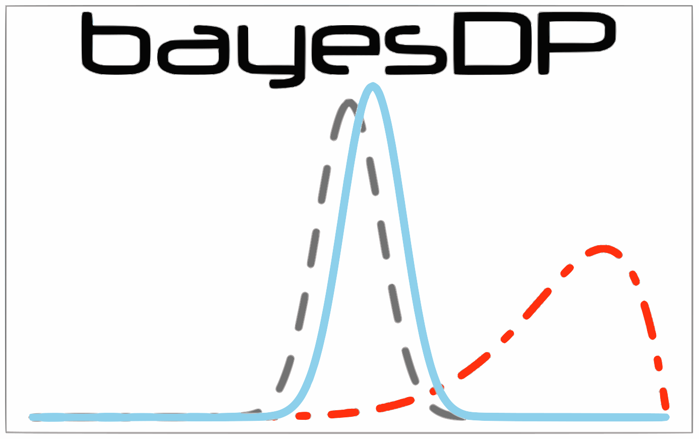
# bayesDP
### Tools for the Bayesian Discount Prior Function
Shiny app available at:
[](https://travis-ci.org/donaldmusgrove/bayesDP)
[](https://codeclimate.com/github/donaldmusgrove/bayesDP)
[](http://www.r-pkg.org/pkg/bayesDP)
[](http://www.repostatus.org/#active)
[](https://github.com/donaldmusgrove/bayesDP/issues)
[](http://www.gnu.org/licenses/gpl-3.0.html)
[](https://cran.r-project.org/package=bayesDP)
### Description
Functions for data augmentation using the Bayesian discount prior
function for 1 arm and 2 arm clinical trials.
### CRAN Installation
Install release version from CRAN:
install.packages("bayesDP")
### GitHub Installation
Install development version from GitHub:
devtools::install_github("donaldmusgrove/bayesDP")
### Documentation
See manuals and vignettes within package.
### Examples
See manuals and vignettes within package.
### Authors
Shawn Balcome, Donnie Musgrove, Tarek Haddad and Christopher Jackson
(For the ppexp R code that was ported to C++.)
### License
GPL (>= 3)
���������������������������������������������������������������������������������������������������������bayesDP/MD5�����������������������������������������������������������������������������������������0000644�0001777�0001777�00000005672�13145350215�013454� 0����������������������������������������������������������������������������������������������������ustar �herbrandt�����������������������herbrandt��������������������������������������������������������������������������������������������������������������������������������������������������������������������������������������������������������������236abbd6e204c61e54cb4b7a51bf0e21 *DESCRIPTION
cbf9702e6372be93c241688bed9cf81e *NAMESPACE
81bbf5bbbd36f970f308223c9f3b8fdd *NEWS.md
86318768a754cf8d76694166035d31e4 *R/RcppExports.R
f347479a08099a9551819021dd02dae8 *R/alpha_discount.R
211e4bfd3433c1ed10cafa9f589ffdbb *R/bdpbinomial.R
6d0bec9d2c3711d19b7e1fb5adae4ce4 *R/bdpnormal.R
9b0417c422980ef1bb849537629ed6d0 *R/bdpregression.R
59e523baa55e3745ddb6ed9ad7a0edad *R/bdpsurvival.R
c6c49955f29748070ba91bc126e98d49 *R/plot.R
51ef880fd11842ded1460318c2386b12 *R/ppexp.R
f75cc4082e711354dea0d2ad6f2ae8aa *R/print.R
32b4168d9f226ca8784541bb9a2d729a *R/probability_discount.R
aa57f793b30a36b3a1f533d2f06361a0 *R/summary.R
d85a2e8bcfc0b11e2aa3a09d96916d2f *README.md
06b47dbc890d6864419d0cd10613a1de *build/vignette.rds
79798a072f8825a096b04324f3a99b17 *inst/doc/bdpbinomial-vignette.R
c35dafa4e2791f0aa18b8275570b2ecd *inst/doc/bdpbinomial-vignette.Rmd
e4be763d8f4da9ea046f2556a7f2d049 *inst/doc/bdpbinomial-vignette.html
8d9a22ccb51ca6c652b7555b2af09706 *inst/doc/bdpnormal-vignette.R
142c8360d112d06c9f09a759dc5527e9 *inst/doc/bdpnormal-vignette.Rmd
d468fc87240006b84c5cf1afa364c52e *inst/doc/bdpnormal-vignette.html
54d68c427c263609e8eff0ddfc19a7ce *inst/doc/bdpsurvival-vignette.R
dd0f7fd90183cb59c112c8e0a6709896 *inst/doc/bdpsurvival-vignette.Rmd
8fe645485f6e3a851febe0f21e73ea0c *inst/doc/bdpsurvival-vignette.html
a47fa6fbe4829cdde8421518dd39f608 *man/alpha_discount.Rd
7d7f0dde09c4df7c2e47212323b4b63d *man/bdpbinomial.Rd
6252469e6ff7c7c42d375304392ff93e *man/bdpnormal.Rd
8a7a0cee19f2cb6d788a92182fca188c *man/bdpregression.Rd
37d802dbe28fc38c263d65f04448ec38 *man/bdpsurvival.Rd
0318c5c79cc39f820a5878dec4c1f661 *man/plot-bdpbinomial-method.Rd
2ba073a545674cc1eca21762b7960b1c *man/plot-bdpnormal-method.Rd
61ec87c7b03573d3405cd8a089418cfd *man/plot-bdpregression-method.Rd
c024a8a2b5701e299e5557816631143f *man/plot-bdpsurvival-method.Rd
fd86dd90585ec28f3110c452b9ea3a96 *man/ppexp.Rd
849b31aa39211b6268297a9531fcf72f *man/print-bdpbinomial-method.Rd
b02a14d96d08df8aa0fb2071a7e56499 *man/print-bdpnormal-method.Rd
a2fe48abba6c921417c0dfebdb821a1c *man/print-bdpregression-method.Rd
1ec913d49f77590d882ec740205065f9 *man/print-bdpsurvival-method.Rd
55cbcc288e4108feea28b8f5ccb28471 *man/probability_discount.Rd
fbd4cbe1090d502e7a2e6cb99aba8071 *man/summary-bdpbinomial-method.Rd
092362fe76dab7c9c50cfbfda1f147df *man/summary-bdpnormal-method.Rd
8e20a77c9c91865da818caa5660b4f41 *man/summary-bdpregression-method.Rd
15f724ea0d2c28a5b732a17a5505b7e0 *man/summary-bdpsurvival-method.Rd
33cdf630eab077900013b8556dbc9cad *src/Makevars
affe08098a93a8eda262515eb58490a0 *src/Makevars.win
e32c57c45ee8e07f62d7b8566f796dd8 *src/RcppExports.cpp
9ca85d31518046064432c4ce0da29a5e *src/bayesDP-init.c
ad77f6196fd91462f1150aa3f1e23402 *src/ppexp.cpp
c35dafa4e2791f0aa18b8275570b2ecd *vignettes/bdpbinomial-vignette.Rmd
142c8360d112d06c9f09a759dc5527e9 *vignettes/bdpnormal-vignette.Rmd
dd0f7fd90183cb59c112c8e0a6709896 *vignettes/bdpsurvival-vignette.Rmd
����������������������������������������������������������������������bayesDP/build/��������������������������������������������������������������������������������������0000755�0001777�0001777�00000000000�13144711751�014236� 5����������������������������������������������������������������������������������������������������ustar �herbrandt�����������������������herbrandt��������������������������������������������������������������������������������������������������������������������������������������������������������������������������������������������������������������bayesDP/build/vignette.rds��������������������������������������������������������������������������0000644�0001777�0001777�00000000435�13144711751�016577� 0����������������������������������������������������������������������������������������������������ustar �herbrandt�����������������������herbrandt���������������������������������������������������������������������������������������������������������������������������������������������������������������������������������������������������������������������������N�0�����l����`������c��C��k����$S�v�ƋCq�����C�8��϶�G]i#�j�m�S���w)�KB$W�P.��NH�V�s�0�[��z�H�d]�����鑂��9�S�i�����v��tA���H= ������*�����������̀(#�%X��t��D�>�I�_'�_��8�u�,a�*������^��������Î�/������~Eۜ[_���f����`>z_��j���������������������������������������������������������������������������������������������������������������������������������������������������������������������������������������������������������������������������������������bayesDP/DESCRIPTION���������������������������������������������������������������������������������0000644�0001777�0001777�00000002420�13145350215�014636� 0����������������������������������������������������������������������������������������������������ustar �herbrandt�����������������������herbrandt��������������������������������������������������������������������������������������������������������������������������������������������������������������������������������������������������������������Package: bayesDP
Type: Package
Title: Tools for the Bayesian Discount Prior Function
Version: 1.2.2
Date: 2017-08-15
Authors@R: c(person("Shawn", "Balcome", email = "sbalcome@mdic.org", role = c("cre")), person("Donnie", "Musgrove", email = "donald.r.musgrove@medtronic.com", role = c("aut")), person("Tarek", "Haddad", email = "tarek.d.haddad@medtronic.com", role = c("aut")), person("Christopher", "Jackson", email = "chris.jackson@mrc-bsu.cam.ac.uk", role = "ctb", comment="For the ppexp R code that was ported to C++."))
Depends: R (>= 3.2.3), ggplot2, survival, methods
Description: Functions for data augmentation using the
Bayesian discount prior function for 1 arm and 2 arm clinical trials.
LazyLoad: yes
License: GPL-3
URL: https://github.com/donaldmusgrove/bayesDP
BugReports: https://github.com/donaldmusgrove/bayesDP/issues
NeedsCompilation: yes
Maintainer: Shawn Balcome
Repository: CRAN
Imports: Rcpp
LinkingTo: Rcpp, RcppArmadillo
RoxygenNote: 6.0.1
Suggests: testthat, knitr, rmarkdown
VignetteBuilder: knitr
Packaged: 2017-08-16 00:38:01 UTC; Shawn Balcome
Author: Shawn Balcome [cre],
Donnie Musgrove [aut],
Tarek Haddad [aut],
Christopher Jackson [ctb] (For the ppexp R code that was ported to
C++.)
Date/Publication: 2017-08-17 17:21:17 UTC
������������������������������������������������������������������������������������������������������������������������������������������������������������������������������������������������������������������������������������������������bayesDP/man/����������������������������������������������������������������������������������������0000755�0001777�0001777�00000000000�13137747566�013731� 5����������������������������������������������������������������������������������������������������ustar �herbrandt�����������������������herbrandt��������������������������������������������������������������������������������������������������������������������������������������������������������������������������������������������������������������bayesDP/man/plot-bdpbinomial-method.Rd��������������������������������������������������������������0000644�0001777�0001777�00000002634�13127770356�020727� 0����������������������������������������������������������������������������������������������������ustar �herbrandt�����������������������herbrandt��������������������������������������������������������������������������������������������������������������������������������������������������������������������������������������������������������������% Generated by roxygen2: do not edit by hand
% Please edit documentation in R/plot.R
\docType{methods}
\name{plot,bdpbinomial-method}
\alias{plot,bdpbinomial-method}
\title{bdpbinomial Object Plot}
\usage{
\S4method{plot}{bdpbinomial}(x, type = NULL, print = TRUE)
}
\arguments{
\item{x}{object of class \code{bdpbinomial}. The result of a call to the
\code{\link{bdpbinomial}} function.}
\item{type}{character. Optional. Select plot type to print.
Supports the following: "discount" gives the discount function;
"posteriors" gives the posterior plots of the event rates; and
"density" gives the augmented posterior density plot(s). Leave NULL to
display all plots in sequence.}
\item{print}{logical. Optional. Produce a plot (\code{print = TRUE}; default) or
return a ggplot object (\code{print = FALSE}). When \code{print = FALSE},
it is possible to use \code{ggplot2} syntax to modify the plot appearance.}
}
\description{
\code{plot} method for class \code{bdpbinomial}.
}
\details{
The \code{plot} method for \code{bdpbinomial} returns up to three
plots: (1) posterior density curves; (2) posterior density of the effect
of interest; and (3) the discount function. A call to \code{plot} that
omits the \code{type} input returns one plot at a time and prompts the
user to click the plot or press return to proceed to the next plot.
Otherwise, the user can specify a plot \code{type} to display the
requested plot.
}
����������������������������������������������������������������������������������������������������bayesDP/man/ppexp.Rd��������������������������������������������������������������������������������0000644�0001777�0001777�00000002517�13127770356�015351� 0����������������������������������������������������������������������������������������������������ustar �herbrandt�����������������������herbrandt��������������������������������������������������������������������������������������������������������������������������������������������������������������������������������������������������������������% Generated by roxygen2: do not edit by hand
% Please edit documentation in R/ppexp.R
\name{ppexp}
\alias{ppexp}
\title{Compute cdf of the piecewise exponential distribution}
\usage{
ppexp(q, x, cuts)
}
\arguments{
\item{q}{scalar. The time point at which the cdf is to be computed.}
\item{x}{vector or matrix. The hazard rate(s).}
\item{cuts}{vector. Times at which the rate changes, i.e., the interval cut
points. The first element of cuts should be 0, and cuts should be in
increasing order. Must be the same length as \code{x} (vector) or have the
same number of columns as \code{x} (matrix)}
}
\value{
The cumulative distribution function computed at time \code{q},
hazard(s) \code{x}, and cut points \code{cuts}.
}
\description{
\code{ppexp} is used to compute the cumulative distribution
function of the piecewise exponential distribution. The function is ported
from R to C++ via code adapted from the \code{msm} package.
}
\details{
The code underlying \code{ppexp} is written in C++ and adapted from
R code used in the \code{msm} package.
}
\examples{
# Single vector of hazard rates. Returns a single cdf value.
q <- 12
x <- c(0.25,0.3,0.35,0.4)
cuts <- c(0,6,12,18)
pp <- ppexp(q,x,cuts)
# Matrix of multiple vectors of hazard rates. Returns 10 cdf values.
x <- matrix(rgamma(4*10, 0.1, 0.1), nrow=10)
pp <- ppexp(q,x,cuts)
}
���������������������������������������������������������������������������������������������������������������������������������������������������������������������������������bayesDP/man/plot-bdpnormal-method.Rd����������������������������������������������������������������0000644�0001777�0001777�00000002614�13127770356�020423� 0����������������������������������������������������������������������������������������������������ustar �herbrandt�����������������������herbrandt��������������������������������������������������������������������������������������������������������������������������������������������������������������������������������������������������������������% Generated by roxygen2: do not edit by hand
% Please edit documentation in R/plot.R
\docType{methods}
\name{plot,bdpnormal-method}
\alias{plot,bdpnormal-method}
\title{bdpnormal Object Plot}
\usage{
\S4method{plot}{bdpnormal}(x, type = NULL, print = TRUE)
}
\arguments{
\item{x}{object of class \code{bdpnormal}. The result of a call to the
\code{\link{bdpnormal}} function.}
\item{type}{character. Optional. Select plot type to print.
Supports the following: "discount" gives the discount function;
"posteriors" gives the posterior plots of the event rates; and
"density" gives the augmented posterior density plot(s). Leave NULL to
display all plots in sequence.}
\item{print}{logical. Optional. Produce a plot (\code{print = TRUE}; default) or
return a ggplot object (\code{print = FALSE}). When \code{print = FALSE},
it is possible to use \code{ggplot2} syntax to modify the plot appearance.}
}
\description{
\code{plot} method for class \code{bdpnormal}.
}
\details{
The \code{plot} method for \code{bdpnormal} returns up to three
plots: (1) posterior density curves; (2) posterior density of the effect
of interest; and (3) the discount function. A call to \code{plot} that
omits the \code{type} input returns one plot at a time and prompts the
user to click the plot or press return to proceed to the next plot.
Otherwise, the user can specify a plot \code{type} to display the
requested plot.
}
��������������������������������������������������������������������������������������������������������������������bayesDP/man/summary-bdpnormal-method.Rd�������������������������������������������������������������0000644�0001777�0001777�00000002664�13127770356�021147� 0����������������������������������������������������������������������������������������������������ustar �herbrandt�����������������������herbrandt��������������������������������������������������������������������������������������������������������������������������������������������������������������������������������������������������������������% Generated by roxygen2: do not edit by hand
% Please edit documentation in R/summary.R
\docType{methods}
\name{summary,bdpnormal-method}
\alias{summary,bdpnormal-method}
\title{bdpnormal Object Summary}
\usage{
\S4method{summary}{bdpnormal}(object)
}
\arguments{
\item{object}{object of class \code{bdpnormal}. The result of a call to the
\code{\link{bdpnormal}} function.}
}
\description{
\code{summary} method for class \code{bdpnormal}.
}
\details{
Displays a summary of the \code{bdpnormal} fit including the
input data, the stochastic comparison between current and historical
data, and the resulting historical data weight (alpha). If historical
data is missing then no stochastic comparison nor weight are displayed.
In the case of a one-arm analysis, the displayed 95 percent
confidence interval contains the lower and upper limits of the
augmented mean value of the current data. The displayed
\code{mean of treatment group} is the mean of the current data
augmented by the historical data.
When a control arm is present, a two-arm analysis is carried out.
Now, the displayed 95 percent confidence interval contains the
lower and upper limits of the difference between the treatment and
control arms with the historical data augmented to current data, if
present. The displayed augmented sample estimates are the
mean of the treatment and control arms, each of
which are augmented when historical data are present.
}
����������������������������������������������������������������������������bayesDP/man/bdpregression.Rd������������������������������������������������������������������������0000644�0001777�0001777�00000021105�13130704536�017044� 0����������������������������������������������������������������������������������������������������ustar �herbrandt�����������������������herbrandt��������������������������������������������������������������������������������������������������������������������������������������������������������������������������������������������������������������% Generated by roxygen2: do not edit by hand
% Please edit documentation in R/bdpregression.R
\name{bdpregression}
\alias{bdpregression}
\alias{bdpregression,ANY-method}
\title{Bayesian Discount Prior: Regression Analysis}
\usage{
bdpregression(formula = formula, family = "gaussian", data = data,
prior_mean = 0, prior_scale = NULL, prior_df = 1,
prior_mean_for_intercept = 0, prior_scale_for_intercept = NULL,
prior_df_for_intercept = 1, alpha_max = 1, fix_alpha = FALSE,
number_mcmc = 10000, weibull_scale = 0.135, weibull_shape = 3,
two_side = TRUE, method = "fixed")
}
\arguments{
\item{formula}{an object of class "formula." See "Details" for
more information, including specfication of historical and treatment
data status.}
\item{family}{a description of the error distribution and link
function to be used in the model. For bdpregression this can
be a character string naming a family function, a family
function or the result of a call to a family function.}
\item{data}{an optional data frame, list or environment
(or object coercible by as.data.frame to a data frame)
containing the variables in the model. If not found in data,
the variables are taken from environment(formula), typically
the environment from which bdpregression is called.}
\item{prior_mean}{prior mean for the coefficients; default is 0.
Can be a vector of length equal to the number of covariates
(not counting the intercept, if any). If it is a scalar, it is
expanded to the length of this vector.}
\item{prior_scale}{prior scale for the coefficients: default is NULL;
if NULL, for a logistic regression model, prior_scale is 2.5; for a
probit model, prior scale is 2.5*1.6. Can be a vector of length equal
to the number of predictors (not counting the intercept, if any). If
it is a scalar, it is expanded to the length of this vector.}
\item{prior_df}{prior degrees of freedom for the coefficients. For
t distribution default is 1 (Cauchy). Set to Inf to get normal prior
distributions. Can be a vector of length equal to the number of
predictors (not counting the intercept, if any). If it is a scalar,
it is expanded to the length of this vector.}
\item{prior_mean_for_intercept}{prior mean for the intercept: default
is 0.}
\item{prior_scale_for_intercept}{prior scale for the intercept:
default is NULL; for a logit model, prior scale for intercept is 10;
for probit model, prior scale for intercept is rescaled as 10*1.6.}
\item{prior_df_for_intercept}{prior degrees of freedom for the
intercept: default is 1.}
\item{alpha_max}{scalar. Maximum weight the discount function can apply.
Default is 1. For a two-arm trial, users may specify a vector of two values
where the first value is used to weight the historical treatment group and
the second value is used to weight the historical control group.}
\item{fix_alpha}{logical. Fix alpha at alpha_max? Default value is FALSE.}
\item{number_mcmc}{scalar. Number of Markov Chain Monte Carlo (MCMC)
simulations. Default is 10000.}
\item{weibull_scale}{scalar. Scale parameter of the Weibull discount function
used to compute alpha, the weight parameter of the historical data. Default
value is 0.135. For a two-arm trial, users may specify a vector of two
values where the first value is used to estimate the weight of the
historical treatment group and the second value is used to estimate the
weight of the historical control group.}
\item{weibull_shape}{scalar. Shape parameter of the Weibull discount function
used to compute alpha, the weight parameter of the historical data. Default
value is 3. For a two-arm trial, users may specify a vector of two values
where the first value is used to estimate the weight of the historical
treatment group and the second value is used to estimate the weight of the
historical control group.}
\item{two_side}{logical. Indicator of two-sided test for the discount
function. Default value is TRUE.}
\item{method}{character. Analysis method with respect to estimation of the weight
paramter alpha. Default value "\code{fixed}" estimates alpha once and holds it fixed
throughout the analysis. Alternative method "\code{mc}" estimates alpha for each
Monte Carlo iteration. Currently, only the default method "\code{fixed}" is
supported.}
}
\value{
\code{bdpregression} returns an object of class "bdpregression".
The functions \code{summary} and \code{print} are used to obtain and
print a summary of the results, including user inputs. The \code{plot}
function displays visual outputs as well.
An object of class "\code{bdpregression}" is a list containing at least
the following components:
\describe{
\item{\code{posterior_treatment}}{
list. Entries contain values related to the treatment group:}
\itemize{
\item{\code{alpha_discount}}{
numeric. Alpha value, the weighting parameter of the historical data.}
\item{\code{p_hat}}{
numeric. The posterior probability of the stochastic comparison
between the current and historical data.}
\item{\code{posterior_regression}}{
list. Contains results for the augmented regression analysis. Entries
are similar to the output of \code{glm} and \code{bayesglm} (from the
\code{arm} package).}
\item{\code{posterior_flat_regression}}{
list. Contains entries similar to \code{posterior_regression} corresponding
to estimates of the unweighted current data.}
\item{\code{prior_regression}}{
to estimates of the historical data.}
}
\item{\code{args1}}{
list. Entries contain user inputs. In addition, the following elements
are ouput:}
\itemize{
\item{\code{df_t} and \code{df_c}}{
dataframe. Input data parsed into internally used treatment and control
data frames.
}
\item{\code{arm2}}{
logical. Used internally to indicate one-arm or two-arm analysis.
}
}
}
}
\description{
\code{bdpregression} is used to estimate the adjusted intercept
(single arm trial; OPC) or treatment effect (two-arm trial; RCT) for
data using the regression analysis implementation of the
Bayesian discount prior.
}
\details{
\code{bdpregression} uses a two-stage approach for determining the
strength of historical data in estimation of an adjusted mean or covariate effect.
In the first stage, a Weibull distribution function is used as a
\emph{discount function} that defines the maximum strength of the
historical data (via \code{weibull_shape}, \code{weibull_scale}, and
\code{alpha_max}) and discounts based on disagreement with the current data.
Disagreement between current and historical data is determined by stochastically
comparing the respective posterior distributions under noninformative priors.
With a single arm regression analysis, the comparison is the
proability (\code{p}) that the current adjusted intercept is less than the
historical adjusted intercept. The comparison metric \code{p} is then
input into the Weibull discount function and the final strength of the
historical data is returned (alpha).
In the second stage, posterior estimation is performed where the discount
function parameter, \code{alpha}, is used as a fixed value for all posterior
estimation procedures.
Two-arm (RCT) analyses are not currently available with this release.
}
\examples{
\dontrun{
# One-arm trial (OPC) example - linear regression
# Simulate regression data for a single arm (OPC) trial
set.seed(3408)
historical <- c(rep(1,50),rep(0,50))
x1 <- c(rnorm(50), rnorm(50))
y <- c(rnorm(50), rnorm(50)+0.2)
fit1 <- bdpregression(y ~ x1 + historical)
summary(fit1)
print(fit1)
plot(fit1, type="discount")
# One-arm trial (OPC) example - logistic regression
set.seed(3408)
historical <- c(rep(1,100),rep(0,100))
x1 <- c(rep(0,50), rep(1,50), rep(0,50), rep(1,50))
y <- rbinom(200,1,plogis(1 + 0.5*x1 + 0.1*historical))
fit2 <- bdpregression(y ~ x1 + historical,
family = binomial)
print(fit2)
# One-arm trial (OPC) example - Poisson regression
set.seed(3408)
historical <- c(rep(1,100),rep(0,100))
x1 <- c(rep(0,50), rep(1,50), rep(0,50), rep(1,50))
y <- rpois(200,exp(1 + 0.5*x1 + 0.5*historical))
fit3 <- bdpregression(y ~ x1 + historical,
family = poisson)
summary(fit3)
# Refit the Poisson data ignoring historical
fit4 <- bdpregression(y ~ x1, family = poisson)
summary(fit4)
# Place data in a dataframe and carry out linear regression
set.seed(3408)
df <- data.frame(historical = c(rep(1,50),rep(0,50)),
x1 = c(rnorm(50), rnorm(50)),
y = c(rnorm(50), rnorm(50)+0.2))
fit5 <- bdpregression(y ~ x1 + historical, data=df)
summary(fit5)
# Two-arm trials are not yet implemented.
}
}
�����������������������������������������������������������������������������������������������������������������������������������������������������������������������������������������������������������������������������������������������������������������������������������������������������������������������������������������������������������������������������������������������������������������������������������������������������������bayesDP/man/summary-bdpregression-method.Rd���������������������������������������������������������0000644�0001777�0001777�00000001405�13127770356�022027� 0����������������������������������������������������������������������������������������������������ustar �herbrandt�����������������������herbrandt��������������������������������������������������������������������������������������������������������������������������������������������������������������������������������������������������������������% Generated by roxygen2: do not edit by hand
% Please edit documentation in R/summary.R
\docType{methods}
\name{summary,bdpregression-method}
\alias{summary,bdpregression-method}
\title{bdpregression Object Summary}
\usage{
\S4method{summary}{bdpregression}(object)
}
\arguments{
\item{object}{object of class \code{bdpregression}. The result of a call to the
\code{\link{bdpregression}} function.}
}
\description{
\code{summary} method for class \code{bdpregression}.
}
\details{
Displays a summary of the \code{bdpregression} fit including the
input data, the stochastic comparison between current and historical
data, and the resulting historical data weight (alpha). If historical
data is missing then no stochastic comparison nor weight are displayed.
...
}
�����������������������������������������������������������������������������������������������������������������������������������������������������������������������������������������������������������������������������������������������������������bayesDP/man/summary-bdpbinomial-method.Rd�����������������������������������������������������������0000644�0001777�0001777�00000002720�13127770356�021442� 0����������������������������������������������������������������������������������������������������ustar �herbrandt�����������������������herbrandt��������������������������������������������������������������������������������������������������������������������������������������������������������������������������������������������������������������% Generated by roxygen2: do not edit by hand
% Please edit documentation in R/summary.R
\docType{methods}
\name{summary,bdpbinomial-method}
\alias{summary,bdpbinomial-method}
\title{bdpbinomial Object Summary}
\usage{
\S4method{summary}{bdpbinomial}(object)
}
\arguments{
\item{object}{object of class \code{bdpbinomial}. The result of a call to the
\code{\link{bdpbinomial}} function.}
}
\description{
\code{summary} method for class \code{bdpbinomial}.
}
\details{
Displays a summary of the \code{bdpbinomial} fit including the
input data, the stochastic comparison between current and historical
data, and the resulting historical data weight (alpha). If historical
data is missing then no stochastic comparison nor weight are displayed.
In the case of a one-arm analysis, the displayed 95 percent
confidence interval contains the lower and upper limits of the
augmented event rate of the current data. The displayed
\code{probability of success} is the event rate of the current data
augmented by the historical data.
When a control arm is present, a two-arm analysis is carried out.
Now, the displayed 95 percent confidence interval contains the
lower and upper limits of the difference between the treatment and
control arms with the historical data augmented to current data, if
present. The displayed augmented sample estimates are the
event rates of the treatment and control arms, each of
which are augmented when historical data are present.
}
������������������������������������������������bayesDP/man/plot-bdpregression-method.Rd������������������������������������������������������������0000644�0001777�0001777�00000001730�13127770356�021311� 0����������������������������������������������������������������������������������������������������ustar �herbrandt�����������������������herbrandt��������������������������������������������������������������������������������������������������������������������������������������������������������������������������������������������������������������% Generated by roxygen2: do not edit by hand
% Please edit documentation in R/plot.R
\docType{methods}
\name{plot,bdpregression-method}
\alias{plot,bdpregression-method}
\title{bdpregression Object Plot}
\usage{
\S4method{plot}{bdpregression}(x, type = NULL, print = TRUE)
}
\arguments{
\item{x}{object of class \code{bdpregression}. The result of a call to the
\code{\link{bdpregression}} function.}
\item{type}{character. Optional. Select plot type to print.
Currently supports "discount", the discount function plot.}
\item{print}{logical. Optional. Produce a plot (\code{print = TRUE}; default) or
return a ggplot object (\code{print = FALSE}). When \code{print = FALSE},
it is possible to use \code{ggplot2} syntax to modify the plot appearance.}
}
\description{
\code{plot} method for class \code{bdpregression}.
}
\details{
The \code{plot} method for \code{bdpregression} currently returns
only the discount function. More plots will be implemented in a future release.
}
����������������������������������������bayesDP/man/summary-bdpsurvival-method.Rd�����������������������������������������������������������0000644�0001777�0001777�00000002744�13127770356�021531� 0����������������������������������������������������������������������������������������������������ustar �herbrandt�����������������������herbrandt��������������������������������������������������������������������������������������������������������������������������������������������������������������������������������������������������������������% Generated by roxygen2: do not edit by hand
% Please edit documentation in R/summary.R
\docType{methods}
\name{summary,bdpsurvival-method}
\alias{summary,bdpsurvival-method}
\title{bdpsurvival Object Summary}
\usage{
\S4method{summary}{bdpsurvival}(object)
}
\arguments{
\item{object}{an object of class \code{bdpsurvival}, a result of a call
to \code{\link{bdpsurvival}}.}
}
\description{
\code{summary} method for class \code{bdpsurvival}.
}
\details{
Displays a summary of the \code{bdpsurvival} fit. The output
is different, conditional on a one- or two-arm survival analysis.
In the case of a one-arm analysis, the stochastic comparison between
current and historical data and the resulting historical data weight
(alpha) are displayed, followed by a survival table containing
augmented posterior estimates of the survival probability at each
time point for the current data.
When a control arm is present, a two-arm analysis is carried out.
A two-arm survival analysis is similar to a cox proportional
hazards analysis, and the displayed summary reflects this. First,
the stochastic comparison between current and historical data and
the resulting historical data weight (alpha) are displayed, when
historical data is present for the respective arm. The displayed
\code{coef} value is the log-hazard between the augmented treatment
and control arms (log(treatment) - log(control)). The lower and upper
95 percent interval limits correspond to the \code{coef} value.
}
����������������������������bayesDP/man/print-bdpsurvival-method.Rd�������������������������������������������������������������0000644�0001777�0001777�00000001702�13127770356�021161� 0����������������������������������������������������������������������������������������������������ustar �herbrandt�����������������������herbrandt��������������������������������������������������������������������������������������������������������������������������������������������������������������������������������������������������������������% Generated by roxygen2: do not edit by hand
% Please edit documentation in R/print.R
\docType{methods}
\name{print,bdpsurvival-method}
\alias{print,bdpsurvival-method}
\title{bdpsurvival Object Print}
\usage{
\S4method{print}{bdpsurvival}(x)
}
\arguments{
\item{x}{object of class \code{bdpsurvival}. The result of a call to the
\code{\link{bdpsurvival}} function.}
}
\description{
\code{print} method for class \code{bdpsurvival}.
}
\details{
Displays a print of the \code{bdpsurvival} fit. The output
is different, conditional on a one- or two-arm survival analysis.
In the case of a one-arm analysis, a brief summary is displayed,
including the current data sample size, number of events,
user input survival time, the augmented median survival probability,
and corresponding lower and upper 95 percent interval limits.
When a control arm is present, the output is the same as a call to
\code{\link[=summary,bdpsurvival-method]{summary}}.
}
��������������������������������������������������������������bayesDP/man/probability_discount.Rd�����������������������������������������������������������������0000644�0001777�0001777�00000004343�13127772200�020432� 0����������������������������������������������������������������������������������������������������ustar �herbrandt�����������������������herbrandt��������������������������������������������������������������������������������������������������������������������������������������������������������������������������������������������������������������% Generated by roxygen2: do not edit by hand
% Please edit documentation in R/probability_discount.R
\name{probability_discount}
\alias{probability_discount}
\alias{probability_discount,ANY-method}
\title{Bayesian Discount Prior: Comparison Between Current and Historical Data}
\usage{
probability_discount(mu = NULL, sigma = NULL, N = NULL, mu0 = NULL,
sigma0 = NULL, N0 = NULL, number_mcmc = 10000, two_side = TRUE)
}
\arguments{
\item{mu}{scalar. Mean of the current data.}
\item{sigma}{scalar. Standard deviation of the current data.}
\item{N}{scalar. Number of observations of the current data.}
\item{mu0}{scalar. Mean of the historical data.}
\item{sigma0}{scalar. Standard deviation of the historical data.}
\item{N0}{scalar. Number of observations of the historical data.}
\item{number_mcmc}{scalar. Number of Monte Carlo simulations. Default is 10000.}
\item{two_side}{logical. Indicator of two-sided test for the discount
function. Default value is TRUE.}
}
\value{
\code{probability_discount} returns an object of class "probability_discount".
An object of class \code{probability_discount} contains the following:
\describe{
\item{\code{p_hat}}{
scalar. The posterior probability of the comparison historical data weight.}
}
}
\description{
\code{probability_discount} can be used to estimate the posterior
probability of the comparison between historical and current data in the
context of a one- or two-arm clinical trial with normal (mean) data.
\code{probability_discount} is not used internally but is
given for educational purposes.
}
\details{
This function is not used internally but is given for educational purposes.
Given the inputs, the output is the posterior probability of the comparison
between current and historical data in the context of a one- or two-arm clinical
trial with normal (mean) data.
}
\examples{
probability_discount(mu = 0, sigma = 1, N = 100,
mu0 = 0.1, sigma0 = 1, N0 = 100)
}
\references{
Haddad, T., Himes, A., Thompson, L., Irony, T., Nair, R. MDIC Computer
Modeling and Simulation working group.(2017) Incorporation of stochastic
engineering models as prior information in Bayesian medical device trials.
\emph{Journal of Biopharmaceutical Statistics}, 1-15.
}
���������������������������������������������������������������������������������������������������������������������������������������������������������������������������������������������������������������������������������������������������������������������������������������������bayesDP/man/print-bdpnormal-method.Rd���������������������������������������������������������������0000644�0001777�0001777�00000001005�13127770356�020572� 0����������������������������������������������������������������������������������������������������ustar �herbrandt�����������������������herbrandt��������������������������������������������������������������������������������������������������������������������������������������������������������������������������������������������������������������% Generated by roxygen2: do not edit by hand
% Please edit documentation in R/print.R
\docType{methods}
\name{print,bdpnormal-method}
\alias{print,bdpnormal-method}
\title{bdpnormal Object Print}
\usage{
\S4method{print}{bdpnormal}(x)
}
\arguments{
\item{x}{object of class \code{bdpnormal}. The result of a call to the
\code{\link{bdpnormal}} function.}
}
\description{
\code{print} method for class \code{bdpnormal}.
}
\details{
Returns same output as a call to \code{\link[=summary,bdpnormal-method]{summary}}.
}
���������������������������������������������������������������������������������������������������������������������������������������������������������������������������������������������������������������������������������������������������������������������������������������������������������������������������������������������������������������������������������������������������������������������������������������������������������������������������������������������������������������������������bayesDP/man/bdpnormal.Rd����������������������������������������������������������������������������0000644�0001777�0001777�00000021650�13127770356�016172� 0����������������������������������������������������������������������������������������������������ustar �herbrandt�����������������������herbrandt��������������������������������������������������������������������������������������������������������������������������������������������������������������������������������������������������������������% Generated by roxygen2: do not edit by hand
% Please edit documentation in R/bdpnormal.R
\name{bdpnormal}
\alias{bdpnormal}
\alias{bdpnormal,ANY-method}
\title{Bayesian Discount Prior: Gaussian mean values}
\usage{
bdpnormal(mu_t = NULL, sigma_t = NULL, N_t = NULL, mu0_t = NULL,
sigma0_t = NULL, N0_t = NULL, mu_c = NULL, sigma_c = NULL,
N_c = NULL, mu0_c = NULL, sigma0_c = NULL, N0_c = NULL,
alpha_max = 1, fix_alpha = FALSE, weibull_scale = 0.135,
weibull_shape = 3, number_mcmc = 10000, two_side = TRUE,
method = "fixed")
}
\arguments{
\item{mu_t}{scalar. Mean of the current treatment group.}
\item{sigma_t}{scalar. Standard deviation of the current treatment group.}
\item{N_t}{scalar. Number of observations of the current treatment group.}
\item{mu0_t}{scalar. Mean of the historical treatment group.}
\item{sigma0_t}{scalar. Standard deviation of the historical treatment
group.}
\item{N0_t}{scalar. Number of observations of the historical treatment
group.}
\item{mu_c}{scalar. Mean of the current control group.}
\item{sigma_c}{scalar. Standard deviation of the current control group.}
\item{N_c}{scalar. Number of observations of the current control group.}
\item{mu0_c}{scalar. Mean of the historical control group.}
\item{sigma0_c}{scalar. Standard deviation of the historical control group.}
\item{N0_c}{scalar. Number of observations of the historical control group.}
\item{alpha_max}{scalar. Maximum weight the discount function can apply.
Default is 1. For a two-arm trial, users may specify a vector of two values
where the first value is used to weight the historical treatment group and
the second value is used to weight the historical control group.}
\item{fix_alpha}{logical. Fix alpha at alpha_max? Default value is FALSE.}
\item{weibull_scale}{scalar. Scale parameter of the Weibull discount function
used to compute alpha, the weight parameter of the historical data. Default
value is 0.135. For a two-arm trial, users may specify a vector of two values
where the first value is used to estimate the weight of the historical
treatment group and the second value is used to estimate the weight of the
historical control group.}
\item{weibull_shape}{scalar. Shape parameter of the Weibull discount function
used to compute alpha, the weight parameter of the historical data. Default
value is 3. For a two-arm trial, users may specify a vector of two values
where the first value is used to estimate the weight of the historical
treatment group and the second value is used to estimate the weight of the
historical control group.}
\item{number_mcmc}{scalar. Number of Monte Carlo simulations. Default is 10000.}
\item{two_side}{logical. Indicator of two-sided test for the discount
function. Default value is TRUE.}
\item{method}{character. Analysis method with respect to estimation of the weight
paramter alpha. Default value "\code{fixed}" estimates alpha once and holds it fixed
throughout the analysis. Alternative method "\code{mc}" estimates alpha for each
Monte Carlo iteration. See the the \code{bdpnormal} vignette \cr
\code{vignette("bdpnormal-vignette", package="bayesDP")} for more details.}
}
\value{
\code{bdpnormal} returns an object of class "bdpnormal". The
functions \code{\link[=summary,bdpnormal-method]{summary}} and
\code{\link[=print,bdpnormal-method]{print}} are used to obtain and print
a summary of the results, including user inputs. The
\code{\link[=plot,bdpnormal-method]{plot}} function displays visual
outputs as well.
An object of class \code{bdpnormal} is a list containing at least
the following components:
\describe{
\item{\code{posterior_treatment}}{
list. Entries contain values related to the treatment group:}
\itemize{
\item{\code{alpha_discount}}{
numeric. Alpha value, the weighting parameter of the historical data.}
\item{\code{p_hat}}{
numeric. The posterior probability of the stochastic comparison
between the current and historical data.}
\item{\code{posterior_mu}}{
vector. A vector of length \code{number_mcmc} containing the posterior
mean of the treatment group. If historical treatment data is present,
the posterior incorporates the weighted historical data.}
\item{\code{posterior_sigma2}}{
vector. A vector of length \code{number_mcmc} containing the posterior
variance of the treatment group. If historical treatment data is present,
the posterior incorporates the weighted historical data.}
\item{\code{posterior_flat_mu}}{
vector. A vector of length \code{number_mcmc} containing
Monte Carlo samples of the mean of the current treatment group
under a flat/non-informative prior, i.e., no incorporation of the
historical data.}
\item{\code{posterior_flat_sigma2}}{
vector. A vector of length \code{number_mcmc} containing
Monte Carlo samples of the standard deviation of the current treatment group
under a flat/non-informative prior, i.e., no incorporation of the
historical data.}
\item{\code{prior_mu}}{
vector. If historical treatment data is present, a vector of length
\code{number_mcmc} containing Monte Carlo samples of the mean
of the historical treatment group under a flat/non-informative prior.}
\item{\code{prior_sigma2}}{
vector. If historical treatment data is present, a vector of length
\code{number_mcmc} containing Monte Carlo samples of the standard deviation
of the historical treatment group under a flat/non-informative prior.}
}
\item{\code{posterior_control}}{
list. Similar entries as \code{posterior_treament}. Only present if a
control group is specified.
}
\item{\code{args1}}{
list. Entries contain user inputs. In addition, the following elements
are ouput:}
\itemize{
\item{\code{arm2}}{
binary indicator. Used internally to indicate one-arm or two-arm
analysis.}
\item{\code{intent}}{
character. Denotes current/historical status of treatment and
control groups.}
}
}
}
\description{
\code{bdpnormal} is used for estimating posterior samples from a
Gaussian outcome where an informative prior is used. The prior weight
is determined using a discount function. This code is modeled after
the methodologies developed in Haddad et al. (2017).
}
\details{
\code{bdpnormal} uses a two-stage approach for determining the
strength of historical data in estimation of a mean outcome. In the first
stage, a Weibull distribution function is used as a
\emph{discount function} that defines the maximum strength of the
historical data (via \code{weibull_shape}, \code{weibull_scale}, and
\code{alpha_max}) and discounts based on disagreement with the current data.
Disagreement between current and historical data is determined by stochastically
comparing the respective posterior distributions under noninformative priors.
With Gaussian data, the comparison is the proability (\code{p}) that the current
mean is less than the historical mean. The comparison metric \code{p} is then
input into the Weibull discount function and the final strength of the
historical data is returned (alpha).
In the second stage, posterior estimation is performed where the discount
function parameter, \code{alpha}, is used as a fixed value for all posterior
estimation procedures.
To carry out a single arm (OPC) analysis, data for the current treatment
(\code{mu_t}, \code{sigma_t}, and \code{N_t}) and historical treatment
(\code{mu0_t}, \code{sigma0_t}, and \code{N0_t}) must be input. The results
are then based on the posterior distribution of the current data augmented
by the historical data.
To carry our a two-arm (RCT) analysis, data for the current treatment and
at least one of current or historical control data must be input.
The results are then based on the posterior distribution of the difference
between current treatment and control, augmented by available historical data.
For more details, see the \code{bdpnormal} vignette: \cr
\code{vignette("bdpnormal-vignette", package="bayesDP")}
}
\examples{
# One-arm trial (OPC) example
fit <- bdpnormal(mu_t = 30, sigma_t = 10, N_t = 250,
mu0_t = 50, sigma0_t = 5, N0_t = 250)
summary(fit)
\dontrun{
plot(fit)
}
# Two-arm (RCT) example
fit2 <- bdpnormal(mu_t = 30, sigma_t = 10, N_t = 250,
mu0_t = 50, sigma0_t = 5, N0_t = 250,
mu_c = 25, sigma_c = 10, N_c = 250,
mu0_c = 50, sigma0_c = 5, N0_c = 250)
summary(fit2)
\dontrun{
plot(fit2)
}
}
\references{
Haddad, T., Himes, A., Thompson, L., Irony, T., Nair, R. MDIC Computer
Modeling and Simulation working group.(2017) Incorporation of stochastic
engineering models as prior information in Bayesian medical device trials.
\emph{Journal of Biopharmaceutical Statistics}, 1-15.
}
\seealso{
\code{\link[=summary,bdpnormal-method]{summary}},
\code{\link[=print,bdpnormal-method]{print}},
and \code{\link[=plot,bdpnormal-method]{plot}} for details of each of the
supported methods.
}
����������������������������������������������������������������������������������������bayesDP/man/print-bdpregression-method.Rd�����������������������������������������������������������0000644�0001777�0001777�00000001024�13127770356�021463� 0����������������������������������������������������������������������������������������������������ustar �herbrandt�����������������������herbrandt��������������������������������������������������������������������������������������������������������������������������������������������������������������������������������������������������������������% Generated by roxygen2: do not edit by hand
% Please edit documentation in R/print.R
\docType{methods}
\name{print,bdpregression-method}
\alias{print,bdpregression-method}
\title{bdpregression Object Print}
\usage{
\S4method{print}{bdpregression}(x)
}
\arguments{
\item{x}{object of class \code{bdpregression}. The result of a call to the
\code{\link{bdpregression}} function.}
}
\description{
\code{print} method for class \code{bdpregression}.
}
\details{
Returns a print of the model with output similar to \code{\link{lm}}.
}
������������������������������������������������������������������������������������������������������������������������������������������������������������������������������������������������������������������������������������������������������������������������������������������������������������������������������������������������������������������������������������������������������������������������������������������������������������������������������������������������������������bayesDP/man/print-bdpbinomial-method.Rd�������������������������������������������������������������0000644�0001777�0001777�00000001025�13127770356�021076� 0����������������������������������������������������������������������������������������������������ustar �herbrandt�����������������������herbrandt��������������������������������������������������������������������������������������������������������������������������������������������������������������������������������������������������������������% Generated by roxygen2: do not edit by hand
% Please edit documentation in R/print.R
\docType{methods}
\name{print,bdpbinomial-method}
\alias{print,bdpbinomial-method}
\title{bdpbinomial Object Print}
\usage{
\S4method{print}{bdpbinomial}(x)
}
\arguments{
\item{x}{object of class \code{bdpbinomial}. The result of a call to the
\code{\link{bdpbinomial}} function.}
}
\description{
\code{print} method for class \code{bdpbinomial}.
}
\details{
Returns same output as a call to
\code{\link[=summary,bdpbinomial-method]{summary}}.
}
�����������������������������������������������������������������������������������������������������������������������������������������������������������������������������������������������������������������������������������������������������������������������������������������������������������������������������������������������������������������������������������������������������������������������������������������������������������������������������������������������������������bayesDP/man/alpha_discount.Rd�����������������������������������������������������������������������0000644�0001777�0001777�00000005256�13127770356�017215� 0����������������������������������������������������������������������������������������������������ustar �herbrandt�����������������������herbrandt��������������������������������������������������������������������������������������������������������������������������������������������������������������������������������������������������������������% Generated by roxygen2: do not edit by hand
% Please edit documentation in R/alpha_discount.R
\name{alpha_discount}
\alias{alpha_discount}
\alias{alpha_discount,ANY-method}
\title{Bayesian Discount Prior: Historical Data Weight (alpha)}
\usage{
alpha_discount(p_hat = NULL, alpha_max = 1, weibull_scale = 0.135,
weibull_shape = 3)
}
\arguments{
\item{p_hat}{scalar. The posterior probability of a stochastic comparison.
This value can be the output of \code{posterior_probability} or a value
between 0 and 1.}
\item{alpha_max}{scalar. Maximum weight the discount function can apply.
Default is 1. For a two-arm trial, users may specify a vector of two values
where the first value is used to weight the historical treatment group and
the second value is used to weight the historical control group.}
\item{weibull_scale}{scalar. Scale parameter of the Weibull discount function
used to compute alpha, the weight parameter of the historical data. Default
value is 0.135. For a two-arm trial, users may specify a vector of two values
where the first value is used to estimate the weight of the historical
treatment group and the second value is used to estimate the weight of the
historical control group.}
\item{weibull_shape}{scalar. Shape parameter of the Weibull discount function
used to compute alpha, the weight parameter of the historical data. Default
value is 3. For a two-arm trial, users may specify a vector of two values
where the first value is used to estimate the weight of the historical
treatment group and the second value is used to estimate the weight of the
historical control group.}
}
\value{
\code{alpha_discount} returns an object of class "alpha_discount".
An object of class \code{alpha_discount} contains the following:
\describe{
\item{\code{alpha_hat}}{
scalar. The historical data weight.
}
}
}
\description{
\code{alpha_discount} can be used to estimate the weight
applied to historical data in the context of a one- or two-arm
clinical trial. \code{alpha_discount} is not used internally but is
given for educational purposes.
}
\details{
This function is not used internally but is given for educational purposes.
Given inputs \code{p_hat}, \code{alpha_max}, \code{weibull_shape}, and
\code{weibull_scale} the output is the weight that would be applied to
historical data in the context of a one- or two-arm clinical trial.
}
\examples{
alpha_discount(0.5)
alpha_discount(0)
}
\references{
Haddad, T., Himes, A., Thompson, L., Irony, T., Nair, R. MDIC Computer
Modeling and Simulation working group.(2017) Incorporation of stochastic
engineering models as prior information in Bayesian medical device trials.
\emph{Journal of Biopharmaceutical Statistics}, 1-15.
}
��������������������������������������������������������������������������������������������������������������������������������������������������������������������������������������������������������������������������������������������������������������������������������������������������������������������������������������������������bayesDP/man/bdpsurvival.Rd��������������������������������������������������������������������������0000644�0001777�0001777�00000025613�13127770356�016560� 0����������������������������������������������������������������������������������������������������ustar �herbrandt�����������������������herbrandt��������������������������������������������������������������������������������������������������������������������������������������������������������������������������������������������������������������% Generated by roxygen2: do not edit by hand
% Please edit documentation in R/bdpsurvival.R
\name{bdpsurvival}
\alias{bdpsurvival}
\alias{bdpsurvival,ANY-method}
\title{Bayesian Discount Prior: Survival Analysis}
\usage{
bdpsurvival(formula = formula, data = data, breaks = NULL, a0 = 0.1,
b0 = 0.1, surv_time = NULL, alpha_max = 1, fix_alpha = FALSE,
number_mcmc = 10000, weibull_scale = 0.135, weibull_shape = 3,
two_side = TRUE, method = "fixed")
}
\arguments{
\item{formula}{an object of class "formula." Must have a survival object on
the left side and exactly two inputs on the right side: treatment and
historical. See "Details" for more information.}
\item{data}{data frame. A data frame with columns 'time', 'status',
'treatment', and historical.' See "Details" for required structure.}
\item{breaks}{vector. Breaks (interval starts) used to compose the breaks of the
piecewise exponential model. Do not include zero. Default breaks are the
quantiles of the input times.}
\item{a0}{scalar. Prior value for the gamma shape of the piecewise
exponential hazards. Default is 0.1.}
\item{b0}{scalar. Prior value for the gamma rate of the piecewise
exponential hazards. Default is 0.1.}
\item{surv_time}{scalar. Survival time of interest for computing the
probability of survival for a single arm (OPC) trial. Default is
overall, i.e., current+historical, median survival time.}
\item{alpha_max}{scalar. Maximum weight the discount function can apply.
Default is 1. For a two-arm trial, users may specify a vector of two values
where the first value is used to weight the historical treatment group and
the second value is used to weight the historical control group.}
\item{fix_alpha}{logical. Fix alpha at alpha_max? Default value is FALSE.}
\item{number_mcmc}{scalar. Number of Monte Carlo simulations. Default is 10000.}
\item{weibull_scale}{scalar. Scale parameter of the Weibull discount function
used to compute alpha, the weight parameter of the historical data. Default
value is 0.135. For a two-arm trial, users may specify a vector of two
values where the first value is used to estimate the weight of the
historical treatment group and the second value is used to estimate the
weight of the historical control group.}
\item{weibull_shape}{scalar. Shape parameter of the Weibull discount function
used to compute alpha, the weight parameter of the historical data. Default
value is 3. For a two-arm trial, users may specify a vector of two values
where the first value is used to estimate the weight of the historical
treatment group and the second value is used to estimate the weight of the
historical control group.}
\item{two_side}{logical. Indicator of two-sided test for the discount
function. Default value is TRUE.}
\item{method}{character. Analysis method with respect to estimation of the weight
paramter alpha. Default value "\code{fixed}" estimates alpha once and holds it fixed
throughout the analysis. Alternative method "\code{mc}" estimates alpha for each
Monte Carlo iteration. See the the \code{bdpsurvival} vignette \cr
\code{vignette("bdpsurvival-vignette", package="bayesDP")} for more details.}
}
\value{
\code{bdpsurvival} returns an object of class "bdpsurvival".
The functions \code{\link[=summary,bdpsurvival-method]{summary}} and \code{\link[=print,bdpsurvival-method]{print}} are used to obtain and
print a summary of the results, including user inputs. The \code{\link[=plot,bdpsurvival-method]{plot}}
function displays visual outputs as well.
An object of class "\code{bdpsurvival}" is a list containing at least
the following components:
\describe{
\item{\code{posterior_treatment}}{
list. Entries contain values related to the treatment group:}
\itemize{
\item{\code{alpha_discount}}{
numeric. Alpha value, the weighting parameter of the historical data.}
\item{\code{p_hat}}{
numeric. The posterior probability of the stochastic comparison
between the current and historical data.}
\item{\code{posterior_survival}}{
vector. If one-arm trial, a vector of length \code{number_mcmc}
containing the posterior probability draws of survival at
\code{surv_time}.}
\item{\code{posterior_flat_survival}}{
vector. If one-arm trial, a vector of length \code{number_mcmc}
containing the probability draws of survival at \code{surv_time}
for the current treatment not augmented by historical treatment.}
\item{\code{prior_survival}}{
vector. If one-arm trial, a vector of length \code{number_mcmc}
containing the probability draws of survival at \code{surv_time}
for the historical treatment.}
\item{\code{posterior_hazard}}{
matrix. A matrix with \code{number_mcmc} rows and \code{length(breaks)}
columns containing the posterior draws of the piecewise hazards
for each interval break point.}
\item{\code{posterior_flat_hazard}}{
matrix. A matrix with \code{number_mcmc} rows and \code{length(breaks)}
columns containing the draws of piecewise hazards for each interval
break point for current treatment not augmented by historical treatment.}
\item{\code{prior_hazard}}{
matrix. A matrix with \code{number_mcmc} rows and \code{length(breaks)}
columns containing the draws of piecewise hazards for each interval break point
for historical treatment.}
}
\item{\code{posterior_control}}{
list. If two-arm trial, contains values related to the control group
analagous to the \code{posterior_treatment} output.}
\item{\code{args1}}{
list. Entries contain user inputs. In addition, the following elements
are ouput:}
\itemize{
\item{\code{S_t}, \code{S_c}, \code{S0_t}, \code{S0_c}}{
survival objects. Used internally to pass survival data between
functions.}
\item{\code{arm2}}{
logical. Used internally to indicate one-arm or two-arm analysis.}
}
}
}
\description{
\code{bdpsurvival} is used to estimate the survival probability
(single arm trial; OPC) or hazard ratio (two-arm trial; RCT) for
right-censored data using the survival analysis implementation of the
Bayesian discount prior. This code is modeled after
the methodologies developed in Haddad et al. (2017).
}
\details{
\code{bdpsurvival} uses a two-stage approach for determining the
strength of historical data in estimation of a survival probability outcome.
In the first stage, a Weibull distribution function is used as a
\emph{discount function} that defines the maximum strength of the
historical data (via \code{weibull_shape}, \code{weibull_scale}, and
\code{alpha_max}) and discounts based on disagreement with the current data.
Disagreement between current and historical data is determined by stochastically
comparing the respective posterior distributions under noninformative priors.
With a single arm survival data analysis, the comparison is the
probability (\code{p}) that the current survival is less than the historical
survival. For a two-arm survival data, analysis the comparison is the
probability that the hazard ratio comparing treatment and control is
different from zero. The comparison metric \code{p} is then
input into the Weibull discount function and the final strength of the
historical data is returned (alpha).
In the second stage, posterior estimation is performed where the discount
function parameter, \code{alpha}, is used as a fixed value for all posterior
estimation procedures.
To carry out a single arm (OPC) analysis, data for the current and
historical treatments are specified in a data frame. The data frame must have
columns with names 'time', 'status', 'treatment', and 'historical.' Column
'time' is the survival (censor) time of the event and 'status' is the
event indicator. The column 'treatment' is used to indicate which observations
are in the treatment and control group. A value of 1 indicates that the
observation is in the treatment group. The column 'historical' indicates
whether the observation is from the historical data (1) or current data (0).
The results are then based on the posterior probability of survival at
\code{surv_time} for the current data augmented by the historical data.
Two-arm (RCT) analyses are specified similarly to a single arm trial. Again
the input data frame must have columns with names 'time', 'status',
'treatment', and 'historical.' Column 'time' is the survival (censor) time
of the event and 'status' is the event indicator. Now, the 'treatment'
column must use 0 to indicate the control group. The current data are
augmented by historical data (if present) and the results are then based
on the posterior distribution of the hazard ratio between the treatment
and control groups.
For more details, see the \code{bdpsurvival} vignette: \cr
\code{vignette("bdpsurvival-vignette", package="bayesDP")}
}
\examples{
# One-arm trial (OPC) example - survival probability at 5 years
# Simulate survival data for a single arm (OPC) trial
time <- c(rexp(50, rate=1/20), rexp(50, rate=1/10))
status <- c(rexp(50, rate=1/30), rexp(50, rate=1/30))
status <- ifelse(time < status, 1, 0)
# Collect data into a data frame
example_surv_1arm <- data.frame(status = status,
time = time,
historical = c(rep(1,50),rep(0,50)),
treatment = 1)
fit1 <- bdpsurvival(Surv(time, status) ~ historical + treatment,
data = example_surv_1arm,
surv_time = 5)
print(fit1)
\dontrun{
plot(fit1)
}
# Two-arm trial (OPC) example
# Simulate survival data for a two-arm trial
time <- c(rexp(50, rate=1/20), # Current treatment
rexp(50, rate=1/10), # Current control
rexp(50, rate=1/30), # Historical treatment
rexp(50, rate=1/5)) # Historical control
status <- rexp(200, rate=1/40)
status <- ifelse(time < status, 1, 0)
# Collect data into a data frame
example_surv_2arm <- data.frame(status = status,
time = time,
historical = c(rep(0,100),rep(1,100)),
treatment = c(rep(1,50),rep(0,50),rep(1,50),rep(0,50)))
fit2 <- bdpsurvival(Surv(time, status) ~ historical + treatment,
data = example_surv_2arm)
summary(fit2)
### Fix alpha at 1
fit2_1 <- bdpsurvival(Surv(time, status) ~ historical + treatment,
data = example_surv_2arm,
fix_alpha = TRUE)
summary(fit2_1)
}
\references{
Haddad, T., Himes, A., Thompson, L., Irony, T., Nair, R. MDIC Computer
Modeling and Simulation working group.(2017) Incorporation of stochastic
engineering models as prior information in Bayesian medical device trials.
\emph{Journal of Biopharmaceutical Statistics}, 1-15.
}
\seealso{
\code{\link[=summary,bdpsurvival-method]{summary}},
\code{\link[=print,bdpsurvival-method]{print}},
and \code{\link[=plot,bdpsurvival-method]{plot}} for details of each of the
supported methods.
}
���������������������������������������������������������������������������������������������������������������������bayesDP/man/bdpbinomial.Rd��������������������������������������������������������������������������0000644�0001777�0001777�00000020047�13127770356�016473� 0����������������������������������������������������������������������������������������������������ustar �herbrandt�����������������������herbrandt��������������������������������������������������������������������������������������������������������������������������������������������������������������������������������������������������������������% Generated by roxygen2: do not edit by hand
% Please edit documentation in R/bdpbinomial.R
\name{bdpbinomial}
\alias{bdpbinomial}
\alias{bdpbinomial,ANY-method}
\title{Bayesian Discount Prior: Binomial counts}
\usage{
bdpbinomial(y_t = NULL, N_t = NULL, y0_t = NULL, N0_t = NULL,
y_c = NULL, N_c = NULL, y0_c = NULL, N0_c = NULL, alpha_max = 1,
fix_alpha = FALSE, a0 = 1, b0 = 1, number_mcmc = 10000,
weibull_scale = 0.135, weibull_shape = 3, two_side = TRUE,
method = "fixed")
}
\arguments{
\item{y_t}{scalar. Number of events for the current treatment group.}
\item{N_t}{scalar. Sample size of the current treatment group.}
\item{y0_t}{scalar. Number of events for the historical treatment group.}
\item{N0_t}{scalar. Sample size of the historical treatment group.}
\item{y_c}{scalar. Number of events for the current control group.}
\item{N_c}{scalar. Sample size of the current control group.}
\item{y0_c}{scalar. Number of events for the historical control group.}
\item{N0_c}{scalar. Sample size of the historical control group.}
\item{alpha_max}{scalar. Maximum weight the discount function can apply.
Default is 1. For a two-arm trial, users may specify a vector of two values
where the first value is used to weight the historical treatment group and
the second value is used to weight the historical control group.}
\item{fix_alpha}{logical. Fix alpha at alpha_max? Default value is FALSE.}
\item{a0}{scalar. Prior value for the beta rate. Default is 1.}
\item{b0}{scalar. Prior value for the beta rate. Default is 1.}
\item{number_mcmc}{scalar. Number of Monte Carlo simulations. Default is 10000.}
\item{weibull_scale}{scalar. Scale parameter of the Weibull discount function
used to compute alpha, the weight parameter of the historical data. Default
value is 0.135. For a two-arm trial, users may specify a vector of two values
where the first value is used to estimate the weight of the historical
treatment group and the second value is used to estimate the weight of the
historical control group.}
\item{weibull_shape}{scalar. Shape parameter of the Weibull discount function
used to compute alpha, the weight parameter of the historical data. Default
value is 3. For a two-arm trial, users may specify a vector of two values
where the first value is used to estimate the weight of the historical
treatment group and the second value is used to estimate the weight of the
historical control group.}
\item{two_side}{logical. Indicator of two-sided test for the discount
function. Default value is TRUE.}
\item{method}{character. Analysis method with respect to estimation of the weight
paramter alpha. Default value "\code{fixed}" estimates alpha once and holds it fixed
throughout the analysis. Alternative method "\code{mc}" estimates alpha for each
Monte Carlo iteration. See the the \code{bdpbinomial} vignette \cr
\code{vignette("bdpbinomial-vignette", package="bayesDP")} for more details.}
}
\value{
\code{bdpbinomial} returns an object of class "bdpbinomial". The
functions \code{\link[=summary,bdpbinomial-method]{summary}} and
\code{\link[=print,bdpbinomial-method]{print}} are used to obtain and
print a summary of the results, including user inputs. The
\code{\link[=plot,bdpbinomial-method]{plot}} function displays visual
outputs as well.
An object of class \code{bdpbinomial} is a list containing at least
the following components:
\describe{
\item{\code{posterior_treatment}}{
list. Entries contain values related to the treatment group:}
\itemize{
\item{\code{alpha_discount}}{
numeric. Alpha value, the weighting parameter of the historical data.}
\item{\code{p_hat}}{
numeric. The posterior probability of the stochastic comparison
between the current and historical data.}
\item{\code{posterior}}{
vector. A vector of length \code{number_mcmc} containing
posterior Monte Carlo samples of the event rate of the treatment
group. If historical treatment data is present, the posterior
incorporates the weighted historical data.}
\item{\code{posterior_flat}}{
vector. A vector of length \code{number_mcmc} containing
Monte Carlo samples of the event rate of the current treatment group
under a flat/non-informative prior, i.e., no incorporation of the
historical data.}
\item{\code{prior}}{
vector. If historical treatment data is present, a vector of length
\code{number_mcmc} containing Monte Carlo samples of the event rate
of the historical treatment group under a flat/non-informative prior.}
}
\item{\code{posterior_control}}{
list. Similar entries as \code{posterior_treament}. Only present if a
control group is specified.}
\item{\code{args1}}{
list. Entries contain user inputs. In addition, the following elements
are ouput:}
\itemize{
\item{\code{arm2}}{
binary indicator. Used internally to indicate one-arm or two-arm
analysis.}
\item{\code{intent}}{
character. Denotes current/historical status of treatment and
control groups.}
}
}
}
\description{
\code{bdpbinomial} is used for estimating posterior samples from a
binomial outcome where an informative prior is used. The prior weight
is determined using a discount function. This code is modeled after
the methodologies developed in Haddad et al. (2017).
}
\details{
\code{bdpbinomial} uses a two-stage approach for determining the
strength of historical data in estimation of a binomial count mean outcome.
In the first stage, a Weibull distribution function is used as a
\emph{discount function} that defines the maximum strength of the
historical data (via \code{weibull_shape}, \code{weibull_scale}, and
\code{alpha_max}) and discounts based on disagreement with the current data.
Disagreement between current and historical data is determined by stochastically
comparing the respective posterior distributions under noninformative priors.
With binomial data, the comparison is the proability (\code{p}) that the current
count is less than the historical count. The comparison metric \code{p} is then
input into the Weibull discount function and the final strength of the
historical data is returned (alpha).
In the second stage, posterior estimation is performed where the discount
function parameter, \code{alpha}, is used as a fixed value for all posterior
estimation procedures.
To carry out a single arm (OPC) analysis, data for the current treatment
(\code{y_t} and \code{N_t}) and historical treatment (\code{y0_t} and
\code{N0_t}) must be input. The results are then based on the posterior
distribution of the current data augmented by the historical data.
To carry our a two-arm (RCT) analysis, data for the current treatment and
at least one of current or historical control data must be input. The results
are then based on the posterior distribution of the difference between
current treatment and control, augmented by available historical data.
For more details, see the \code{bdpbinomial} vignette: \cr
\code{vignette("bdpbinomial-vignette", package="bayesDP")}
}
\examples{
# One-arm trial (OPC) example
fit <- bdpbinomial(y_t = 10,
N_t = 500,
y0_t = 25,
N0_t = 250)
summary(fit)
print(fit)
\dontrun{
plot(fit)
}
# Two-arm (RCT) example
fit2 <- bdpbinomial(y_t = 10,
N_t = 500,
y0_t = 25,
N0_t = 250,
y_c = 8,
N_c = 500,
y0_c = 20,
N0_c = 250)
summary(fit2)
print(fit2)
\dontrun{
plot(fit2)
}
}
\references{
Haddad, T., Himes, A., Thompson, L., Irony, T., Nair, R. MDIC Computer
Modeling and Simulation working group.(2017) Incorporation of stochastic
engineering models as prior information in Bayesian medical device trials.
\emph{Journal of Biopharmaceutical Statistics}, 1-15.
}
\seealso{
\code{\link[=summary,bdpbinomial-method]{summary}},
\code{\link[=print,bdpbinomial-method]{print}},
and \code{\link[=plot,bdpbinomial-method]{plot}} for details of each of the
supported methods.
}
�����������������������������������������������������������������������������������������������������������������������������������������������������������������������������������������������������������������������������������������������������������������������������������������������������������������������������������������������������������������������������������������������������������������������������������������������������������������������������������������bayesDP/man/plot-bdpsurvival-method.Rd��������������������������������������������������������������0000644�0001777�0001777�00000002430�13127770356�021002� 0����������������������������������������������������������������������������������������������������ustar �herbrandt�����������������������herbrandt��������������������������������������������������������������������������������������������������������������������������������������������������������������������������������������������������������������% Generated by roxygen2: do not edit by hand
% Please edit documentation in R/plot.R
\docType{methods}
\name{plot,bdpsurvival-method}
\alias{plot,bdpsurvival-method}
\title{bdpsurvival Object Plot}
\usage{
\S4method{plot}{bdpsurvival}(x, type = NULL, print = TRUE)
}
\arguments{
\item{x}{object of class \code{bdpsurvival}. The result of a call to the
\code{\link{bdpsurvival}} function.}
\item{type}{character. Optional. Select plot type to print.
Supports the following: "discount" gives the discount function and
"survival" gives the survival curves. Leave NULL to
display all plots in sequence.}
\item{print}{logical. Optional. Produce a plot (\code{print = TRUE}; default) or
return a ggplot object (\code{print = FALSE}). When \code{print = FALSE},
it is possible to use \code{ggplot2} syntax to modify the plot appearance.}
}
\description{
\code{plot} method for class \code{bdpsurvival}.
}
\details{
The \code{plot} method for \code{bdpsurvival} returns up to two
plots: (1) posterior survival curves and (2) the discount function. A
call to \code{plot} that omits the \code{type} input returns one plot
at a time and prompts the user to click the plot or press return to
proceed to the next plot. Otherwise, the user can specify a plot
\code{type} to display the requested plot.
}
��������������������������������������������������������������������������������������������������������������������������������������������������������������������������������������������������������������������������������������������������������������������������������������������������������������������������������������������������������������������������������������������������������������������������������������������������������������������������������������������������������������������������������������������������������������������������������������������������������������������������������������������������������������������������������������������������������������������������������������������������������������������������������������������������������������������������������������������������������������������������������������������������������������������������������������������������������������������������������������������������������������������������������������������������������������������������������������������������������������������������������������������������������������������������������������������������������������������������������������������������������������������������������������������������������������������������������������������������������������������������������������������������������������������������������������������������������������������������������������������������������������������������������������������������������������������������������������������������������������������������������������������������������������������������������������������������������������������������������������������������������������������������������������������������������������������������������������������������������������������������������������������������������������������������������������������������������������������������������������������������������������������������������������������������������������������������������������������������������������������������������������������������������������������������������������������������������������������������������������������������������������������������������������������������������������������������������������������������������������������������������������������������������������������������������������������������������������������������������������������������������������������������������������������������������������������������������������������������������������������������������������������������������������������������������������������������������������������������������������������������������������������������������������������������������������������������������������������������������������������������������������������������������������������������������������������������������������������������������������������������������������������������������������������������������������������������������������������������������������������������������������������������������������������������������������������������������������������������������������������������������������������������������������������������������������������������������������������������������������������������������������������������������������������������������������������������������������������������������������������������������������������������������������������������������������������������������������������������������������������������������������������������������������������������������������������������������������������������������������������������������������������������������������������������������������������������������������������������������������������������������������������������������������������������������������������������������������������������������������������������������������������������������������������������������������������������������������������������������������������������������������������������������������������������������������������������������������������������������������������������������������������������������������������������������������������������������������������������������������������������������������������������������������������������������������������������������������������������������������������������������������������������������������������������������������������������������������������������������������������������������������������������������������������������������������������������������������������������������������������������������������������������������������������������������������������������������������������������������������������������������������������������������������������������������������������������������������������������������������������������������������������������������������������������������������������������������������������������������������������������������������������������������������������������������������������������������������������������������������������������������������������������������������������������������������������������������������������������������������������������������������������������������������������������������������������������������������������������������������������������������������������������������������������������������������������������������������������������������������������������������������������������������������������������������������������������������������������������������������������������������������������������������������������������������������������������������������������������������������������������������������������������������������������������������������������������������������������������������������������������������������������������������������������������������������������������������������������������������������������������������������������������������������������������������������������������������������������������������������������������������������������������������������������������������������������������������������������������������������������������������������������������������������������������������������������������������������������������������������������������������������������������������������������������������������������������������������������������������������������������������������������������������������������������������������������������������������������������������������������������������������������������������������������������������������������������������������������������������������������������������������������������������������������������������������������������������������������������������������������������������������������������������������������������������������������������������������������������������������������������������������������������������������������������������������������������������������������������������������������������������������������������������������������������������������������������������������������������������������������������������������������������������������������������������������������������������������������������������������������������������������������������������������������������������������������������������������������������������������������������������������������������������������������������������������������������������������������������������������������������������������������������������������������������������������������������������������������������������������������������������������������������������������������������������������������������������������������������������������������������������������������������������������������������������������������������������������������������������������������������������������������������������������������������������������������������������������������������������������������������������������������������������������������������������������������������������������������������������������������������������������������������������������������������������������������������������������������������������������������������������������������������������������������������������������������������������������������������������������������������������������������������������������������������������������������������������������������������������������������������������������������������������������������������������������������������������������������������������������������������������������������������������������������������������������������������������������������������������������������������������������������������������������������������������������������������������������������������������������������������������������������������������������������������������������������������������������������������������������������������������������������������������������������������������������������������������������������������������������������������������������������������������������������������������������������������������������������������������������������������������������������������������������������������������������������������������������������������������������������������������������������������������������������������������������������������������������������������������������������������������������������������������������������������������������������������������������������������������������������������������������������������������������������������������������������������������������������������������������������������������������������������������������������������������������������������������������������������������������������������������������������������������������������������������������������������������������������������������������������������������������������������������������������������������������������������������������������������������������������������������������������������������������������������������������������������������������������������������������������������������������������������������������������������������������������������������������������������������������������������������������������������������������������������������������������������������������������������������������������������������������������������������������������������������������������������������������������������������������������������������������������������������