


The hardware and bandwidth for this mirror is donated by METANET, the Webhosting and Full Service-Cloud Provider.
If you wish to report a bug, or if you are interested in having us mirror your free-software or open-source project, please feel free to contact us at mirror[@]metanet.ch.
The DiscreteMorseR package delivers ultra-fast C++ backend Morse gradient field and critical simplices (0-simplices: vertices, 1-simplices: edges, 2-simplices: faces) parallel computation. Perfect for LiDAR data, computational topology, and Morse theory applications.
# From CRAN (once available - recommended)
install.packages("DiscreteMorseR")

# ahull3D and lidR are not on CRAN - install from GitHub
remotes::install_github("DijoG/ahull3D")
remotes::install_github("r-lidar/lidR")

# For development version from GitHub
# remotes::install_github("DijoG/DiscreteMorseR")

# Install recommended dependencies
install.packages(c("Rcpp", "data.table", "dplyr", "purrr", "stringr"))

library(DiscreteMorseR)
Quick test of C++ functions
DiscreteMorseR::get_MIXEDSORT_cpp(c("2", "1", "12 45", "25 256", "11 8", "256 23"))
DiscreteMorseR::add_DECIMAL(215.2585589, 3)Rcpp - C++ integrationdata.table - Fast data operationsdplyr, purrr, stringr - Data
manipulationggplot2, patchwork - Visualizationclustermq - Parallel processing backendtictoc - Timing benchmarkslibrary(lidR)
library(tidyverse)
library(data.table)
library(ahull3D)
# Load LiDAR data
laz_file <- system.file("extdata", "12trees.laz", package = "ahull3D")
trees <- lidR::readLAS(laz_file)
lidR::plot(trees, pal = "grey98")
# Create matrix input for alpha hull
lasdf <-
trees@data[, c("X", "Y", "Z", "pid")] %>%
as.data.frame() %>%
distinct(X, Y, Z, .keep_all = TRUE) %>%
as.matrix()
# Generate alpha hull
a <- ahull3D::ahull3D(lasdf[,1:3],
input_truth = lasdf[,4],
alpha = .1)
# Extract largest connected component mesh
mesh <- DiscreteMorseR::get_CCMESH(a)Real-world computation on tree point cloud (226,267 vertices):
tictoc::tic()
morse_complex <- DiscreteMorseR::compute_MORSE_complex(
  mesh,
  output_dir = "12_output",
  cores = 12,
  batch_size = 5000  # Increase for large datasets
)
tictoc::toc()
# ~2.5 minutes for typical TLS tree point clouds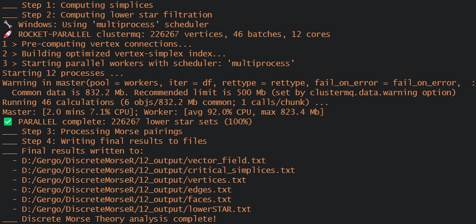
🚀 Performance Highlights: - ✅ 226,267
vertices processed in parallel
- ✅ 12 cores utilized (~92% CPU efficiency) - ✅
100% completion rate - all lower star sets computed -
✅ Complete Morse analysis in ~2.5 minutes - ✅
Automatic file export of all results
crit_types <- sapply(strsplit(morse_complex$critical, " "), length)
table(crit_types)
# 1 = vertices (0-simplices, minima), 2 = edges (1-simplices), 3 = faces (2-simplices)
crit_types
     1      2      3
225137 115 1005 # Critical simplices only: XZ projection
p <- DiscreteMorseR::visualize_MORSE_2d(
morse_complex,
projection = "XZ",
point_alpha = .6,
point_size = .8,
plot_gradient = FALSE,
max_points = 30000
)
print(p)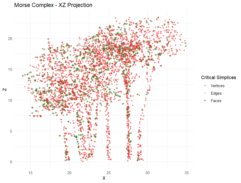
# Critical simplices only: XY projection
pp <- DiscreteMorseR::visualize_MORSE_2d(
  morse_complex,
  projection = "XY",
  point_alpha = .6,
  point_size = .8,
  plot_gradient = FALSE,
  max_points = 30000
)
print(pp)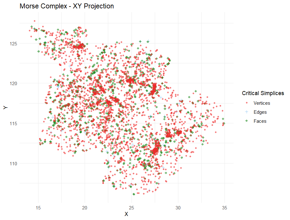
These binaries (installable software) and packages are in development.
They may not be fully stable and should be used with caution. We make no claims about them.