The hardware and bandwidth for this mirror is donated by METANET, the Webhosting and Full Service-Cloud Provider.
If you wish to report a bug, or if you are interested in having us mirror your free-software or open-source project, please feel free to contact us at mirror[@]metanet.ch.
adrftools is an R package for estimating the average
dose-response function (ADRF), which characterizes the effect of a
continuous treatment on an outcome. Functionality is included for
performing g-computation on a regression model to estimate the ADRF,
plot the ADRF, and test hypotheses about the ADRF. See
vignette("adrftools") for a full tutorial on using
adrftools.
You can install the current stable version of adrftools from CRAN with:
install.packages("adrftools")You can install the development version of adrftools from GitHub with:
# install.packages("pak")
pak::pak("ngreifer/adrftools")Below we use adrftools to estimate and characterize the effect of blood lead levels on scores on a cognitive test, adjusting for potential confounders using g-computation.
library(adrftools)

data("nhanes3lead")
Here, the treatment is logBLL, the outcome is
Math, and the confounders to be adjusted for are
Age, Male, Race,
PIR, Enough_Food, Smoke_in_Home,
Smoke_Pregnant, and NICU. We’ll first fit an
outcome model that adjusts for these confounders.
fit <- lm(Math ~ splines::ns(logBLL, df = 5) *
            (Age + Race + Male + PIR + Enough_Food +
               Smoke_in_Home + Smoke_Pregnant + NICU),
          data = nhanes3lead)
Next we’ll use adrftools::adrf() to compute the
ADRF.
adrf_bll <- adrf(fit, treat = "logBLL")

adrf_bll
#> An <effect_curve> object
#>
#> - curve type: ADRF
#> - response: Math
#> - treatment: logBLL
#> + range: -0.3567 to 2.4248
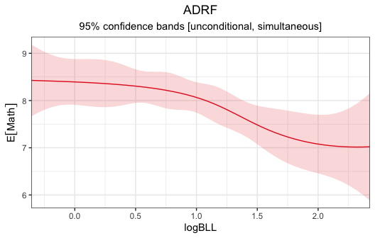
#> - inference: unconditionalWe can plot the ADRF using plot():
plot(adrf_bll)
By default, this produces simultaneous 95% confidence bands.
adrf_bll is an <effect_curve> object,
which is a function. We can supply to it values of the treatment to
compute the corresponding value of the ADRF at those treatment
values:
adrf_bll(logBLL = c(0, .5, 1, 1.5, 2))#> ADRF Estimates
#> ────────────────
#> logBLL Estimate
#> 0.0 8.394
#> 0.5 8.305
#> 1.0 8.066
#> 1.5 7.484
#> 2.0 7.078
#> ────────────────We can also produce confidence intervals using summary()
on the above output:
adrf_bll(logBLL = c(0, .5, 1, 1.5, 2)) |>
  summary()
#> ADRF Estimates
#> ──────────────────────────────────────────
#> logBLL Estimate Std. Error CI Low CI High
#> 0.0 8.394 0.1706 7.959 8.829
#> 0.5 8.305 0.1247 7.987 8.623
#> 1.0 8.066 0.1129 7.778 8.354
#> 1.5 7.484 0.1436 7.117 7.850
#> 2.0 7.078 0.2186 6.520 7.635
#> ──────────────────────────────────────────
#> Inference: unconditional, simultaneous
#> Confidence level: 95% (t* = 2.55, df = 2455)To test an omnibus hypothesis about the ADRF, such as whether it is
flat or linear, we can use summary() on the
<effect_curve> object itself:
# Test for flatness
summary(adrf_bll, hypothesis = "flat")
#> Omnibus Curve Test
#> ───────────────────────────────────────────────────────
#> H₀: ADRF is flat for values of logBLL between -0.3567
#> and 2.4248
#>
#> P-value
#> < 0.0001
#> ───────────────────────────────────────────────────────
#> Computed using the Imhof approximation# Test for linearity
summary(adrf_bll, hypothesis = "linear")#> Omnibus Curve Test
#> ───────────────────────────────────────────────────────
#> H₀: ADRF is linear for values of logBLL between
#> -0.3567 and 2.4248
#>
#> P-value
#> 0.3159
#> ───────────────────────────────────────────────────────
#> Computed using the Imhof approximationThe results indicate that the ADRF is not flat, but there isn’t enough evidence to claim it is nonlinear in the range specified. We might project a linear model onto the ADRF to produce a more interpretable summary:
proj <- curve_projection(adrf_bll, model = "linear")Below, we plot the linear projection along with the original ADRF:
plot(adrf_bll, proj = proj)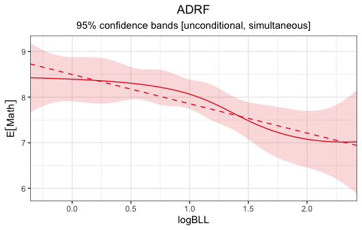
To examine the coefficient describing the projection, we can use
summary() on the projection:
summary(proj)#> ADRF Projection Coefficients
#> ──────────────────────────────────────────────────────────────
#> Term Estimate Std. Error t P-value CI Low CI High
#> (Intercept) 8.498 0.1329 63.96 < 0.0001 8.237 8.758
#> logBLL -0.642 0.1266 -5.07 < 0.0001 -0.891 -0.394
#> ──────────────────────────────────────────────────────────────
#> Inference: unconditional
#> Confidence level: 95% (t* = 1.961, df = 2455)
#> Null value: 0Based on the above, we might conclude the following:
There is some relationship between
logBLLandMathadjusting for the included potential confounders, based on rejection of the hypothesis that the ADRF is flat forlogBLLvalues between -0.3567 and 2.4248 (p < .0001). There isn’t evidence that the ADRF is nonlinear within this range (p = .3153). The linear projection has a coefficient of -.643 (p < .0001), indicating that the expected potential outcome ofMathdecreases by this amount for each unit increase inlogBLL.
See vignette("adrftools") for more information on how to
use adrftools and the other features available.
These binaries (installable software) and packages are in development.
They may not be fully stable and should be used with caution. We make no claims about them.