The hardware and bandwidth for this mirror is donated by METANET, the Webhosting and Full Service-Cloud Provider.
If you wish to report a bug, or if you are interested in having us mirror your free-software or open-source project, please feel free to contact us at mirror[@]metanet.ch.

avstrat

Stratigraphic Data Processing and Section Plots

This package provides tools for data processing and generating stratigraphic sections for volcanic deposits and tephrastratigraphy. Package was developed for studies on Alaska volcanoes (“av”) where stratigraphic (“strat”) figures are needed for interpreting eruptive histories, but the methods are applicable to any sediment stratigraphy project. The primary outputs are ggplot figures of stratigraphic sections–ggstrat(), ggstrat_column(), ggstrat_sampleID()-but the data processing logic add_depths() and add_layer_widths() enable motivated users to create custom visualizations. Various load_data functions facilitate ingesting from stratigraphic layer data templates.

Installation

You can install avstrat from CRAN or from a downloaded source file off the GitLab approved repository (Code - Download source code - tar.gz). For option 2, you’ll need to download the source repo as a tar.gz and map the path to the location on your computer (replace “path/to” with the file path on your local computer where you save the download).

{r eval=FALSE}
# Option 1: Install from CRAN:
install.packages("avstrat")

# Option 2: Install from source file:
install.packages("path/to/avstrat_0.0.0.9000.tar.gz", repos = NULL, type = "source")

To install the development version, use the ‘devtools’ package.

devtools::install_gitlab("vsc/tephra/tools/avstrat", 
                        host = "code.usgs.gov", 
                        build_vignettes = TRUE)

You can also install the development version from a mirrored repo on Github.

devtools::install_github(
  "https://github.com/mwloewen/avstrat",
  build_vignettes = TRUE
)

Example

To upload data from GeoDIVA submission templates (Stations-Samples and Layers), you will need to have two excel files that match GeoDIVA upload templates. Examples can be found in this repo under inst/extdata/example_layers_upload_2024.xlsx and inst/extdata/example_samples_stations_upload_2024.xlsx. In the code chunk below, replace “path_layers.xlsx” with the file path and file name of your files.

library(readxl)
library(avstrat)

data_strat <- load_geodiva_forms(
   station_sample_upload = 
     readxl::read_excel("path/to/samples_stations_upload.xlsx", sheet = "Data"),
   layer_upload = 
     readxl::read_excel("path/to/layers_upload.xlsx", sheet = "Data")
 )

The GeoDIVA templates have some idiosyncrasies unique to Alaska Volcano Observatory projects and database history. Most people may find a more generic upload template more useful, and there is an upload function for that too! See inst/extdata/example_inputs.xlsx, which includes data tabs broken down into different data types: stations, sections, layers, and samples. These can be partially merged (e.g., “stations_sections”) or separate. Samples can be linked to layers as a nested list (similar to the GeoDIVA layer upload, “layers-sample”) or each sample linked to a single layer (“samples_layer”). Using the later option:

data_strat <- load_stratdata_indiv(
  stations_upload = readxl::read_xlsx("path/to/example_inputs.xlsx", 
                                      sheet = "stations"),
  sections_upload = readxl::read_xlsx("path/to/example_inputs.xlsx", 
                                      sheet = "sections"),
  layers_upload = readxl::read_xlsx("path/to/example_inputs.xlsx", 
                                      sheet = "layers"),
  samples_upload = readxl::read_xlsx("path/to/example_inputs.xlsx", 
                                      sheet = "samples_layer"),
)

Once you have the data in your environment, you can make a basic stratigraphic plot and use the avstrat theme:

library(ggplot2)
#> Warning: package 'ggplot2' was built under R version 4.4.3
library(readxl)
#> Warning: package 'readxl' was built under R version 4.4.3
library(avstrat)
# Load data (this is a pre-loaded example dataset that is part of avstrat)
data_strat <- example_data_strat

# Set theme
theme_set(theme_avstrat())

# Produce a strat section
ggstrat(df = data_strat, section_name = '21LSHD02')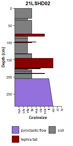

You can also plot sample identification along side the section. and combine them with the patchwork package.

library(patchwork)
#> Warning: package 'patchwork' was built under R version 4.4.3
p1 <- ggstrat(df = data_strat, section_name = '21LSHD02')
p2 <- ggstrat_label(df = data_strat, section_name = '21LSHD02')

p1 + p2
#> Warning in grid.Call.graphics(C_text, as.graphicsAnnot(x$label), x$x, x$y, :
#> font family not found in Windows font database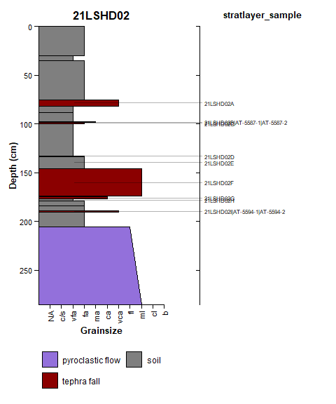

More examples and demonstration of how to create your own custom plots will be provided [eventually] in vignettes! Currently, a more detailed workflow can be accessed with the installed package at:

vignette("avstrat-workflow-examples", package = "avstrat")

Contributing

If you find problems with this package or have features you’d like to see, please open an issue or consider contributing yourself, I would love to have more contributors to the package!

License and Disclaimer

License: This project is in the public domain.

Disclaimer: This software is preliminary or provisional and is subject to revision.

These binaries (installable software) and packages are in development.
They may not be fully stable and should be used with caution. We make no claims about them.