
The hardware and bandwidth for this mirror is donated by METANET, the Webhosting and Full Service-Cloud Provider.
If you wish to report a bug, or if you are interested in having us mirror your free-software or open-source project, please feel free to contact us at mirror[@]metanet.ch.
![]()
![]()

It maps viridis colours (by default) to values, and quickly!
Note It does not perform a 1-to-1 mapping of a palette to values. It interpolates the colours from a given palette.
I’m aware there are other methods for mapping colours to values. And
which do it quick too. But I can never remember them, and I find the
interfaces a bit cumbersome. For example,
scales::col_numeric(palette = viridisLite::viridis(5), domain = range(1:5))(1:5).
I wanted one function which will work on one argument.
colour_values(1:5)
# [1] "#440154FF" "#3B528BFF" "#21908CFF" "#5DC963FF" "#FDE725FF"
colour_values(letters[1:5])
# [1] "#440154FF" "#3B528BFF" "#21908CFF" "#5DC963FF" "#FDE725FF"
I also want it available at the src (C/C++) level for
linking to other packages.
Because it’s correct, and R tells us to
For consistency, aim to use British (rather than American) spelling
But don’t worry, color_values(1:5) works as well
From CRAN
install.packages("colourvalues")Or install the development version from GitHub with:
# install.packages("devtools")
devtools::install_github("SymbolixAU/colourvalues")Rcpp
All functions are written in Rcpp. I have exposed some
of them in header files so you can “link to” them in your package.
For example, the LinkingTo section in
DESCRIPTION will look something like
LinkingTo:
    Rcpp,
    colourvalues
And in a c++ source file so you can
#include the API header
#include "colourvalues/api.hpp"
// [[Rcpp::depends(colourvalues)]]
And call
// return hex colours
colourvalues::api::colour_values_hex()

// return RGP matrix
colourvalues::api::colour_values_rgb()
R
If you’re not using Rcpp, just Import this
package like you would any other.
Of course!
bar_plot <- function(df) {
  barplot( height = df[["a"]], col = df[["col"]], border = NA, space = 0, yaxt = 'n')
}
df <- data.frame(a = 10, x = 1:256)
df$col <- colour_values(df$x, palette = "viridis")
bar_plot( df )
df <- data.frame(a = 10, x = c((1:5000)**3))
df$col <- colour_values(df$x, palette = "viridis")
bar_plot( df )
df <- data.frame(a = 10, x = rnorm(n = 1000))
df$col <- colour_values(df$x, palette = "inferno")
bar_plot( df )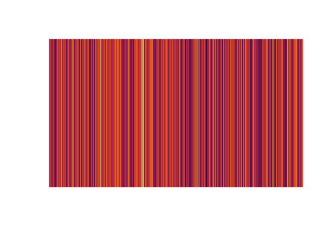
Eurgh!
df <- df[with(df, order(x)), ]
bar_plot( df )
That’s better!
No, you can chose one from
colour_palettes()
#  [1] "viridis"        "cividis"        "magma"          "inferno"
#  [5] "plasma"         "ylorrd"         "ylorbr"         "ylgnbu"
#  [9] "ylgn"           "reds"           "rdpu"           "purples"
# [13] "purd"           "pubugn"         "pubu"           "orrd"
# [17] "oranges"        "greys"          "greens"         "gnbu"
# [21] "bupu"           "bugn"           "blues"          "spectral"
# [25] "rdylgn"         "rdylbu"         "rdgy"           "rdbu"
# [29] "puor"           "prgn"           "piyg"           "brbg"
# [33] "terrain"        "topo"           "heat"           "cm"
# [37] "rainbow"        "terrain_hcl"    "heat_hcl"       "sequential_hcl"
# [41] "rainbow_hcl"    "diverge_hcl"    "diverge_hsv"    "ygobb"
# [45] "matlab_like2"   "matlab_like"    "magenta2green"  "cyan2yellow"
# [49] "blue2yellow"    "green2red"      "blue2green"     "blue2red"
And you can use show_colours() to view them all. Here’s
what some of them look like
show_colours( colours = colour_palettes(c("viridis", "colorspace")))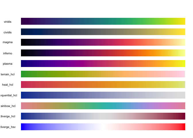
No, you can use your own specified as a matrix of red, green and blue columns in the range [0,255]
n <- 100
m <- grDevices::colorRamp(c("red", "green"))( (1:n)/n )
df <- data.frame(a = 10, x = 1:n)
df$col <- colour_values(df$x, palette = m)
bar_plot( df )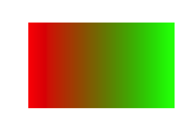
Yep. Either supply a single alpha value for all the colours
## single alpha value for all colours
df <- data.frame(a = 10, x = 1:255)
df$col <- colour_values(df$x, alpha = 50)
bar_plot( df )
Or use a vector of values the same length as x
df <- data.frame(a = 10, x = 1:300, y = rep(c(1:50, 50:1), 3) )
df$col <- colour_values(df$x, alpha = df$y)
bar_plot( df )
Or include the alpha value as a 4th column in the palette matrix
n <- 100
m <- grDevices::colorRamp(c("red", "green"))( (1:n)/n )
## alpha values
m <- cbind(m, seq(0, 255, length.out = 100))
df <- data.frame(a = 10, x = 1:n)
df$col <- colour_values(df$x, palette = m)
bar_plot( df )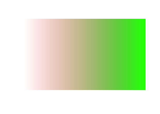
Yep. Set include_alpha = FALSE
colour_values(1:5, include_alpha = F)
# [1] "#440154" "#3B528B" "#21908C" "#5DC963" "#FDE725"
colour_values_rgb(1:5, include_alpha = F)
#      [,1] [,2] [,3]
# [1,]   68    1   84
# [2,]   59   82  139
# [3,]   33  144  140
# [4,]   93  201   99
# [5,] 253 231 37Yes, for numeric values use the n_summaries argument to
specify the number of summary values you’d like
colour_values(1:10, n_summaries = 3)
# $colours
#  [1] "#440154FF" "#482878FF" "#3E4A89FF" "#31688EFF" "#26838EFF" "#1F9D89FF"
#  [7] "#35B779FF" "#6CCE59FF" "#B4DD2CFF" "#FDE725FF"
#
# $summary_values
# [1] "1.00"  "5.50"  "10.00"
#
# $summary_colours
# [1] "#440154FF" "#21908CFF" "#FDE725FF"
You can also specify the number of digits you’d like returned in the summary
colour_values(rnorm(n = 10), n_summaries = 3, digits = 2)
# $colours
#  [1] "#FDE725FF" "#440154FF" "#5CC863FF" "#3F4889FF" "#443A83FF" "#1E9D89FF"
#  [7] "#1E9C89FF" "#77D153FF" "#4EC36BFF" "#2D718EFF"
#
# $summary_values
# [1] "-1.27" "0.36"  "1.99"
#
# $summary_colours
# [1] "#440154FF" "#21908CFF" "#FDE725FF"
You can also use format = FALSE if you don’t want the
summary values formatted.
dte <- seq(as.Date("2018-01-01"), as.Date("2018-02-01"), by = 1)
colour_values(dte, n_summaries = 3)
# $colours
#  [1] "#440154FF" "#470D60FF" "#48196BFF" "#482474FF" "#472E7CFF" "#453882FF"
#  [7] "#414286FF" "#3E4B8AFF" "#3A548CFF" "#365D8DFF" "#32658EFF" "#2E6D8EFF"
# [13] "#2B758EFF" "#287D8EFF" "#25858EFF" "#228C8DFF" "#20948CFF" "#1E9C89FF"
# [19] "#20A386FF" "#25AB82FF" "#2DB27DFF" "#39BA76FF" "#48C16EFF" "#58C765FF"
# [25] "#6ACD5BFF" "#7ED34FFF" "#92D742FF" "#A8DB34FF" "#BEDF26FF" "#D4E21BFF"
# [31] "#E9E41AFF" "#FDE725FF"
#
# $summary_values
# [1] "2018-01-01" "2018-01-16" "2018-02-01"
#
# $summary_colours
# [1] "#440154FF" "#21908CFF" "#FDE725FF"

colour_values(dte, n_summaries = 3, format = F)
# $colours
#  [1] "#440154FF" "#470D60FF" "#48196BFF" "#482474FF" "#472E7CFF" "#453882FF"
#  [7] "#414286FF" "#3E4B8AFF" "#3A548CFF" "#365D8DFF" "#32658EFF" "#2E6D8EFF"
# [13] "#2B758EFF" "#287D8EFF" "#25858EFF" "#228C8DFF" "#20948CFF" "#1E9C89FF"
# [19] "#20A386FF" "#25AB82FF" "#2DB27DFF" "#39BA76FF" "#48C16EFF" "#58C765FF"
# [25] "#6ACD5BFF" "#7ED34FFF" "#92D742FF" "#A8DB34FF" "#BEDF26FF" "#D4E21BFF"
# [31] "#E9E41AFF" "#FDE725FF"
#
# $summary_values
# [1] 17532.0 17547.5 17563.0
#
# $summary_colours
# [1] "#440154FF" "#21908CFF" "#FDE725FF"
For categorical values use summary = TRUE to return a
uniqe set of the values, and their associated colours
colour_values(sample(letters, size = 50, replace = T), summary = T)
# $colours
#  [1] "#277F8EFF" "#63CB5FFF" "#63CB5FFF" "#1FA187FF" "#3C4F8AFF" "#365C8DFF"
#  [7] "#FDE725FF" "#365C8DFF" "#1FA187FF" "#471365FF" "#365C8DFF" "#DFE318FF"
# [13] "#238A8DFF" "#3C4F8AFF" "#80D34DFF" "#46327FFF" "#35B779FF" "#471365FF"
# [19] "#440154FF" "#26AC81FF" "#1FA187FF" "#2C748EFF" "#63CB5FFF" "#FDE725FF"
# [25] "#80D34DFF" "#46327FFF" "#1F968BFF" "#BFDF25FF" "#3C4F8AFF" "#2C748EFF"
# [31] "#9FDA3AFF" "#31688EFF" "#4AC26DFF" "#4AC26DFF" "#3C4F8AFF" "#4AC26DFF"
# [37] "#35B779FF" "#9FDA3AFF" "#1FA187FF" "#26AC81FF" "#482374FF" "#1F968BFF"
# [43] "#26AC81FF" "#FDE725FF" "#4AC26DFF" "#3C4F8AFF" "#277F8EFF" "#35B779FF"
# [49] "#80D34DFF" "#424186FF"
#
# $summary_values
#  [1] "b" "c" "d" "e" "f" "g" "h" "i" "j" "k" "m" "n" "o" "p" "q" "r" "s" "u" "v"
# [20] "w" "x" "y"
#
# $summary_colours
#  [1] "#440154FF" "#471365FF" "#482374FF" "#46327FFF" "#424186FF" "#3C4F8AFF"
#  [7] "#365C8DFF" "#31688EFF" "#2C748EFF" "#277F8EFF" "#238A8DFF" "#1F968BFF"
# [13] "#1FA187FF" "#26AC81FF" "#35B779FF" "#4AC26DFF" "#63CB5FFF" "#80D34DFF"
# [19] "#9FDA3AFF" "#BFDF25FF" "#DFE318FF" "#FDE725FF"Basically, it’s the same as un-listing the list to create a vector of all the values, then colouring them.
So if your list contains different types, it will coerce all values to the same type and colour them.
But it returns a list of the same structure.
For example,
l <- list( x = 1:5, y = list(z = letters[1:5] ) )
colour_values( l )
# [[1]]
# [1] "#440154FF" "#482878FF" "#3E4A89FF" "#31688EFF" "#26838EFF"
#
# [[2]]
# [[2]][[1]]
# [1] "#1F9D89FF" "#35B779FF" "#6CCE59FF" "#B4DD2CFF" "#FDE725FF"

x <- c( 1:5, letters[1:5] )
colour_values( x )
#  [1] "#440154FF" "#482878FF" "#3E4A89FF" "#31688EFF" "#26838EFF" "#1F9D89FF"
#  [7] "#35B779FF" "#6CCE59FF" "#B4DD2CFF" "#FDE725FF"
What it doesn’t do is treat each list element independently. For this you would use
lapply( l, colour_values )
# $x
# [1] "#440154FF" "#3B528BFF" "#21908CFF" "#5DC963FF" "#FDE725FF"
#
# $y
# $y[[1]]
# [1] "#440154FF" "#3B528BFF" "#21908CFF" "#5DC963FF" "#FDE725FF"10 million numeric values
library(microbenchmark)
library(scales)
library(viridisLite)

n <- 1e7
df <- data.frame(x = rnorm(n = n))

m <- microbenchmark(
  colourvalues = { colourvalues::colour_values(x = df$x) },
  scales = { col_numeric(palette = rgb(subset(viridis.map, opt=="D")[, 1:3]), domain = range(df$x))(df$x) },
  times = 25
)
# Warning in microbenchmark(colourvalues = {: less accurate nanosecond times to
# avoid potential integer overflows
m
# Unit: milliseconds
#          expr       min        lq      mean    median        uq       max neval
#  colourvalues  789.3592  797.2215  808.1314  805.4144  810.2691  866.7162    25
#        scales 1696.3621 1761.6745 1820.4097 1793.3245 1865.7442 2118.4543    25
1 million characters (26 unique values)
library(microbenchmark)
library(scales)
library(viridisLite)

n <- 1e6
x <- sample(x = letters, size = n, replace = TRUE)
df <- data.frame(x = x)

m <- microbenchmark(
  colourvalues = { x <- colourvalues::colour_values(x = df$x) },
  scales = { y <- col_factor(palette = rgb(subset(viridis.map, opt=="D")[, 1:3]), domain = unique(df$x))(df$x) },
  times = 25
)
m
# Unit: milliseconds
#          expr       min        lq      mean    median        uq      max neval
#  colourvalues  90.27962  90.81623  91.88558  90.93574  91.61257 104.2933    25
#        scales 195.65930 198.46062 203.90773 200.45052 204.15282 228.5454    25
These binaries (installable software) and packages are in development.
They may not be fully stable and should be used with caution. We make no claims about them.