| Type: | Package |
| Title: | Integrated Camera-Trap Data Management and Analysis |
| Version: | 0.4.0 |
| Date: | 2026-06-20 |
| Imports: | activity (≥ 1.3.4), dplyr (≥ 1.1.4), camtrapdp, cli (≥ 3.6.3), Distance (≥ 2.0.0), ggplot2 (≥ 3.5.2), lubridate, magrittr (≥ 2.0.3), methods, overlap (≥ 0.3.9), rlang (≥ 1.1.5), sbd (≥ 0.1.0), sf (≥ 1.0-19), terra (≥ 1.8-29), tibble, tidyr (≥ 1.3.1), tidyselect, Rcpp (≥ 1.0.14) |
| Maintainer: | Stanislas Mahussi Gandaho <stangandaho@gmail.com> |
| Description: | An integrated, tidyverse-friendly workflow for camera trap data in wildlife monitoring and ecological research. Reads and edits media metadata, filters independent detections, analyses activity patterns and species diversity, and estimates species density or abundance with several methods, including the random encounter model, camera-trap distance sampling, time-to-event, space-to-event, and the random encounter and staying-time model (see Rowcliffe et al. (2008) <doi:10.1111/j.1365-2664.2008.01473.x>, Howe et al. (2017) <doi:10.1111/2041-210X.12790>, Nakashima et al. (2018) <doi:10.1111/1365-2664.13059>, and Moeller et al. (2018) <doi:10.1002/ecs2.2331>). |
| License: | MIT + file LICENSE |
| Encoding: | UTF-8 |
| LazyData: | true |
| RoxygenNote: | 7.3.2 |
| Suggests: | assertr, iNEXT (≥ 3.0.2), httr2, kableExtra (≥ 1.4.0), knitr (≥ 1.50), leaflet (≥ 2.2.2), MASS, MCMCvis, msm, nimble, coda, progress, rmarkdown, shiny (≥ 1.10.0), testthat (≥ 3.0.0), vegan (≥ 2.6-6.1), xml2 |
| Config/testthat/edition: | 3 |
| URL: | https://stangandaho.github.io/ct/ |
| BugReports: | https://github.com/stangandaho/ct/issues |
| Depends: | R (≥ 3.5) |
| Config/Needs/website: | rmarkdown |
| LinkingTo: | Rcpp |
| NeedsCompilation: | yes |
| Packaged: | 2026-07-07 17:39:17 UTC; ganda |
| Author: | Stanislas Mahussi Gandaho
 [aut, cre],
Pablo Palencia
[ctb, rev],
R Consortium [fnd] [aut, cre],
Pablo Palencia
[ctb, rev],
R Consortium [fnd] |
| Repository: | CRAN |
| Date/Publication: | 2026-07-16 13:10:08 UTC |
ct: Integrated Camera-Trap Data Management and Analysis
Description

An integrated, tidyverse-friendly workflow for camera trap data in wildlife monitoring and ecological research. Reads and edits media metadata, filters independent detections, analyses activity patterns and species diversity, and estimates species density or abundance with several methods, including the random encounter model, camera-trap distance sampling, time-to-event, space-to-event, and the random encounter and staying-time model (see Rowcliffe et al. (2008) doi:10.1111/j.1365-2664.2008.01473.x, Howe et al. (2017) doi:10.1111/2041-210X.12790, Nakashima et al. (2018) doi:10.1111/1365-2664.13059, and Moeller et al. (2018) doi:10.1002/ecs2.2331).
Author(s)
Maintainer: Stanislas Mahussi Gandaho stangandaho@gmail.com (ORCID)
Other contributors:
Pablo Palencia palencia.pablo.m@gmail.com (ORCID) [contributor, reviewer]
R Consortium [funder]
See Also
Useful links:
Pipe operators
Description
Re-exported from the magrittr package. %>% pipes the left-hand side
into the first argument (or the . placeholder) of the right-hand side;
%<>% does the same but assigns the result back to the left-hand side.
Usage
lhs %>% rhs

lhs %<>% rhs
Arguments
lhs |
A value to pipe into the right-hand side expression. |
rhs |
A function call using the magrittr semantics; the value of |
Value
The result of calling rhs with lhs inserted, as documented in
magrittr::%>%(). %<>% returns that result invisibly after assigning it
back to lhs.
Camera trap dataset from Agbogon Community Biological Reserve (ACBR), Benin
Description
A curated camera trap dataset from the Agonve Community Wetland Reserve in West Africa, adapted from Gandaho et al. (2026). The dataset contains wildlife camera trap observations and associated deployment metadata.
Format
A named list with two tibbles:
acbr_dataCamera trap observations.
deploymentDeployment metadata.
Details
The object is provided as a named list with two elements:
acbr_data-
A tibble containing camera trap observations.
Variables include:
imageImage file name.
deploymentDeployment identifier.
camCamera station identifier.
modelCamera model (
RD1003LorTC302445).datesObservation date.
timesObservation time.
speciesRecorded species name.
countNumber of individuals detected.
datetimeCombined date-time in POSIX format.
deployment-
A tibble containing deployment-level metadata.
Variables include:
deploymentDeployment identifier.
camCamera station identifier.
modelCamera model.
startDeployment start date-time.
endDeployment end date-time.
radiusCamera detection radius (meters).
angleCamera detection angle (degrees).
areaEstimated detection area (square meters).
The deployment table was reconstructed from the observation data using the first and last timestamps recorded for each deployment.
References
Gandaho, S. M., Agossou, H., Madokoun, D. L., Hounnouvi, E. F. K., Oussoukpevi, S. J. K., Akpona, H. A., Thompson, L., & Djagoun, C. A. M. S. (2026). Habitat loss and species diel ecology in a West African community wetland reserve. Zenodo. doi:10.5281/zenodo.19662320
Examples
data(ACBR)

# Access observation data
head(ACBR$acbr_data)

# Access deployment metadata
head(ACBR$deployment)
Determine the Per-User Directory for R Package Data, Config, or Cache
Description
Determine the per-user directory where packages can store data, configuration files, or caches.
Usage
R_user_dir(package, which = c("data", "config", "cache"))
Arguments
package |
Character string giving the package name. |
which |
Character string specifying the directory type.
Must be one of |
Value
A character string giving the full path to the package-specific per-user directory.
Calculate active periods for camera trap data
Description
Internal helper function to calculate continuous active periods based on gap detection.
Usage
calc_active_periods(data, threshold, time_unit)
Arguments
data |
A data frame containing the datetime column. |
threshold |
A numeric value indicating the minimum gap to be considered a break (default is 10). |
time_unit |
The unit for the threshold. Supported values include "secs", "mins", "hours", "days", and "weeks". |
Value
A tibble with period_start and period_end columns.
Compute QAIC for a set of detection function models
Description
Calculates the quasi-Akaike Information Criterion (QAIC) for one or more detection function models within the same key function family. If multiple models are provided, all must have the same key function. This function is typically used as the first step of a two-step model selection approach (Howe et al., 2019).
Usage
ct_QAIC(models, chat = NULL, k = 2)
Arguments
models |
A list of fitted detection function models (objects returned by
|
chat |
Optional numeric value of overdispersion ( |
k |
Numeric. The penalty term used in QAIC (default is |
Details
If only one model is supplied and chat is not provided, the function
estimates \hat{c} using the provided model and issues a warning that
model selection cannot be performed. For multiple models, All models must use the same key function.
QAIC is calculated as:
QAIC = -2 \times \log(L) / \hat{c} + 2k
where L is the likelihood, \hat{c} is the estimated
overdispersion, and k is the number of parameters.
Value
A tibble with one row per model containing:
-
model: The model name -
df: The degrees of freedom for the model. -
QAIC: The computed QAIC value.
References
Howe, E. J., Buckland, S. T., Després-Einspenner, M., & Kühl, H. S. (2019). Model selection with overdispersed distance sampling data. Methods in Ecology and Evolution, 10(1), 38-47. doi:10.1111/2041-210X.13082
Examples
library(Distance)
library(dplyr)

data("duiker")
duiker_data <- duikers$DaytimeDistances %>%
  dplyr::slice_sample(prop = .3) # sample 30% of rows
truncation <- list(left = 2, right = 15) # Keep only distance between 2-15 m

# fit hazard-rate key models
w3_hr0 <- ds(duiker_data, transect = "point", key = "hr", adjustment = NULL,
             truncation = truncation)
w3_hr1 <- ds(duiker_data, transect = "point", key = "hr", adjustment = "cos",
             order = 2, truncation = truncation)
w3_hr2 <- ds(duiker_data, transect = "point", key = "hr", adjustment = "cos",
             order = c(2, 4), truncation = truncation)
# fit half-normal key models
w3_hn0 <- ds(duiker_data, transect = "point", key = "hn", adjustment = NULL,
             truncation = truncation)
w3_hn1 <- ds(duiker_data, transect = "point", key = "hn", adjustment = "cos",
             order = 2, truncation = truncation)
w3_hn2 <- ds(duiker_data, transect = "point", key = "hn", adjustment = "cos",
             order = c(2, 4), truncation = truncation)
# fit uniform key models
w3_u0 <- ds(duiker_data, transect = "point", key = "unif", adjustment = NULL,
            truncation = truncation)
w3_u1 <- ds(duiker_data, transect = "point", key = "unif", adjustment = "cos",
            order = 2, truncation = truncation)
w3_u2 <- ds(duiker_data, transect = "point", key = "unif", adjustment = "cos",
            order = c(2, 4), truncation = truncation)

# Create model list
model_list <- list(w3_hn0, w3_hn1, w3_hn2,
                   w3_hr0, w3_hr1, w3_hr2,
                   w3_u0, w3_u1, w3_u2)

# Compute model QAICs
ct_QAIC(list(w3_hr0, w3_hr1, w3_hr2)) # All key functions must be the same
ct_QAIC(list(w3_hn0, w3_hn1, w3_hn2)) # All key functions must be the same

# Compute Chi-squared Goodness-of-fit
ct_chi2_select(list(w3_hn0, w3_hr0, w3_u0)) # All key functions must be different
ct_chi2_select(list(w3_hn2, w3_hr1, w3_u0)) # All key functions must be different

# Two-step model selection
ct_select_model(model_list)
Alpha diversity index
Description
Calculate index diversity within a particular area or ecosystem; usually expressed by the number of species (i.e., species richness) in that ecosystem.
Usage
ct_alpha_diversity(
  data,
  to_community = TRUE,
  index = "shannon",
  site_column,
  species_column,
  size_column = NULL,
  margin = 1
)
Arguments
data |
A data frame containing species observation data. |
to_community |
Logical; if |
index |
A character vector specifying the diversity index to calculate.
Accepted values are |
site_column |
The column name in |
species_column |
The column(s) in |
size_column |
(Optional) The column in |
margin |
An integer specifying whether diversity calculations should be
performed by row ( |
Details
Simpson diversity index
Simpson (1949) introduced a diversity index that quantifies the likelihood of two randomly chosen individuals belonging to the same species. This probability increases as diversity decreases; in a scenario with no diversity (only one species), the probability reaches 1. Simpson's Index is computed using the following formula:
D = \sum_{i=1}^{S} \left( \frac{n_{i}}{N} \right)^2
where n_{i} is the number of individuals in species i,
N = total number of individuals of all species, and \frac{n_{i}}{N} = pi
(proportion of individuals of species i), and S = species richness.
The value of Simpson's D ranges from 0 to 1, with 0 representing infinite
diversity and 1 representing no diversity, so the larger the value of D,
the lower the diversity. For this reason, Simpson's index is often as its
complement (1-D). Simpson's Dominance Index is the inverse of the
Simpson's Index (1/D).
Shannon-Weiner Diversity Index
Shannon-Weiner Diversity Index is a measure of diversity that takes into account both species richness and evenness, introduced by Claude Shannon in 1948. Commonly referred to as Shannon's Diversity Index, it is based on the concept of uncertainty. For instance, in a community with very low diversity, there is a high level of certainty (or low uncertainty) about the identity of a randomly selected organism. Conversely, in a highly diverse community, the uncertainty increases, making it harder to predict which species a randomly chosen organism will belong to (low certainty or high uncertainty).
H = -\sum_{i=1}^{S} p_{i} * \ln p_{i}
where p_{i} = proportion of individuals of species i, and ln is the natural logarithm,
and S = species richness. The value of H ranges from 0 to Hmax.
Hmax is different for each community and depends on species richness.
(Note: Shannon-Weiner is often denoted H' ).
Pielou or Evenness diversity index
Species evenness refers to the relative abundance of each species within an environment. For example, if there are 40 foxes and 1000 dogs, the community is uneven because one species dominates. However, if there are 40 foxes and 42 dogs, the community is much more even, as the species are more balanced in number. The degree of evenness in a community can be quantified using Pielou's evenness index (Pielou, 1966):
J=\frac{H}{H_{\max }}
The value of J ranges from 0 to 1. Higher values indicate higher levels of evenness. At maximum evenness, J = 1. J and D can be used as measures of species dominance (the opposite of diversity) in a community. Low J indicates that 1 or few species dominate the community.
Value
A tibble with diversity index values for each site.
The first column corresponds to site_column, followed by one or more columns containing
the computed diversity indices, depending on the values specified in the index argument.
References
Pielou, E.C. (1966). The measurement of diversity in different types of biological collections. Journal of Theoretical Biology, 13, pp. 131-144. doi:10.1016/0022-5193(66)90013-0.
Simpson, E.H. (1949). Measurement of diversity. Nature, 163, pp. 688. doi:10.1038/163688a0
Shannon, C.E. (1948). A mathematical theory of communication. The Bell System Technical Journal, 27, pp. 379-423.doi:10.1002/j.1538-7305.1948.tb01338.x
Examples
data(penessoulou)
cam_data <- penessoulou %>%
  dplyr::filter(project == "Last")

# Transform data to community format and compute diversity indices
alpha1 <- cam_data %>%
  ct_alpha_diversity(
    to_community = TRUE,
    size_column = number,
    site_column = camera,
    species_column = species,
    index = c("shannon", "evenness", "invsimpson")
  )

# Alternative method using a manually transformed community matrix
alpha2 <- cam_data %>%
  ct_to_community(site_column = camera, species_column = species,
                  size_column = number, values_fill = 0) %>%
  ct_alpha_diversity(
    to_community = FALSE,
    site_column = camera,
    species_column = 2:11,
    index = c("shannon", "evenness", "invsimpson")
  )
alpha2
# Compare results
all(alpha1 == alpha2) # TRUE
Temporal availability adjustment
Description
Calculates availability correction factors by accounting for temporal variation in animal activity patterns and camera deployment effort. The availability rate represents the proportion of time animals are available for detection (Rowcliffe, et al., 2014; Howe et al., 2017) given their activity patterns and camera sampling effort.
Usage
ct_availability(
  times,
  format = NULL,
  sample = c("data", "model"),
  n_bootstrap = 1000,
  cam_daily_effort = 24,
  ...
)
Arguments
times |
Vector of detection times, either in radians (0 - |
format |
Time format string (e.g., "%H:%M:%S", "%H:%M") if times need conversion to radians. Set to NULL if times are already in radians. |
sample |
Character string defining sampling method for bootstrapping errors (see details). |
n_bootstrap |
Number of bootstrap iterations to perform. Ignored if sample=="none" |
cam_daily_effort |
Daily operational hours of cameras (default = 24 for continuous operation). |
... |
Arguments passed on to
|
Value
A list containing data frame with:
-
rate: Estimated availability rate (0-1) -
SE: Standard error of the availability rate
References
Howe, E. J., Buckland, S. T., Després-Einspenner, M. L., & Kühl, H. S. (2017). Distance sampling with camera traps. Methods in Ecology and Evolution, 8(11), 1558-1565. doi:10.1111/2041-210X.12790
Rowcliffe, J. M., Kays, R., Kranstauber, B., Carbone, C., & Jansen, P. A. (2014). Quantifying levels of animal activity using camera trap data. Methods in Ecology and Evolution, 5(11), 1170-1179. doi:10.1111/2041-210X.12278
See Also
Examples
# Example with times already in radians
radian_times <- c(1.2, 3.4, 5.1, 0.5, 2.8)
ct_availability(radian_times, sample = "data")

# Example with formatted times
time_strings <- c("06:30", "18:15", "12:00", "23:45")
ct_availability(time_strings, sample = "data", format = "%H:%M")

# With bootstrap resampling
ct_availability(radian_times, sample = "data", n_bootstrap = 100)
Bootstrap confidence intervals
Description
Confidence interval calculation from bootstrap samples.
Usage
ct_boot_ci(t0, bt, conf = 0.95)
Arguments
t0 |
the statistic estimated from the original sample, usually the output from |
bt |
a vector of bootstrap statistics, usually the output from |
conf |
a (single!) confidence interval to estimate. |
Value
A numeric matrix of confidence limits, as returned by
overlap::bootCI(). Each row corresponds to one of the estimators supplied
in t0 and the two columns give the lower and upper bounds of the
confidence interval at the requested level (conf).
Generate bootstrap estimates of overlap
Description
The function takes two sets of times of observations and calculates bootstrap
estimates of the chosen estimator of overlap. Alternatively, bootstrap
estimates can be calculated in a 2-stage process: (1) create a matrix of
bootstrap samples for each data set, using ct_resample(); (2) pass these
matrices to ct_boot_estimates() to obtain the bootstrap estimates.
A vector of bootstrap estimates can then be used to produce confidence intervals
with ct_boot_ci().
Usage
ct_bootstrap(
  A,
  B,
  nb,
  smooth = TRUE,
  kmax = 3,
  adjust = NA,
  n_grid = 128,
  type = c("Dhat1", "Dhat4", "Dhat5"),
  cores = 1
)

ct_resample(x, nb, smooth = TRUE, kmax = 3, adjust = 1, n_grid = 512)

ct_boot_estimates(
  Amat,
  Bmat,
  kmax = 3,
  adjust = c(0.8, 1, 4),
  n_grid = 128,
  type = c("all", "Dhat1", "Dhat4", "Dhat5"),
  cores = 1
)
Arguments
A |
A numeric vector of time-of-day observations (in radians, 0 to |
B |
A numeric vector of time-of-day observations (in radians, 0 to |
nb |
the number of bootstrap samples required |
smooth |
if TRUE, smoothed bootstrap samples are produced. |
kmax |
An integer indicating the maximum number of modes allowed in the activity pattern. Default is 3. |
adjust |
A numeric value to adjust the bandwidth of the kernel density estimation. Default is 1. |
n_grid |
An integer specifying the number of grid points for density estimation. Default is 128. |
type |
the name of the estimator to use, or "all" to produce all three
estimates. See |
cores |
the number of cores to use for parallel processing. If NA, all but one of the available cores will used. Parallel processing may take longer than serial processing if the bootstrap runs quickly. |
x |
a numeric vector of time-of-capture data in radians, ie. on [0, |
Amat, Bmat |
matrices of resampled data for each species produced by |
Value
The function ct_bootstrap() returns a vector of bootstrap estimates.
If estimation fails for a bootstrap sample, the corresponding value will be NA.
The function ct_resample() returns a numeric matrix with each column corresponding
to a bootstrap sample. Times are in radians. It may return a matrix of NAs if
smooth = TRUE and bandwidth estimation fails.
The Function ct_boot_estimates() with type = "all" returns a numeric matrix
with three columns, one for each estimator of overlap, otherwise a vector of
bootstrap estimates.
Author(s)
Mike Meredith, Martin Ridout.
References
Ridout & Linkie (2009) Estimating overlap of daily activity patterns from camera trap data. Journal of Agricultural, Biological, and Environmental Statistics 14:322-337
See Also
Examples
# Generate random data for two species
set.seed(42)
species_A <- runif(100, 1.2, 2 * pi)
species_B <- runif(100, 0.23, 2 * pi)

est <- ct_overlap_estimates(species_A, species_B, type="Dhat4")

boots <- ct_bootstrap(species_A, species_B, 100, type="Dhat4", cores=1)
mean(boots)
hist(boots)
ct_boot_ci(est, boots)

# alternatively:
species_A_gen <- ct_resample(species_A, 100)
species_B_gen <- ct_resample(species_B, 100)
boots <- ct_boot_estimates(species_A_gen, species_B_gen, type="Dhat4", cores=1)
mean(boots)
Calculate daily camera trap captures
Description
Aggregates camera trap data into daily capture summaries.
Usage
ct_camera_day(
  data,
  deployment_data = NULL,
  deployment_column,
  datetime_column,
  species_column,
  size_column,
  format,
  start_column = NULL,
  end_column = NULL,
  deployment_format = format,
  time_zone = ""
)
Arguments
data |
A data frame containing camera trap observation data. |
deployment_data |
A data frame containing camera trap deployment records. |
deployment_column |
The column name (unquoted or as a string) that uniquely identifies the deployment (e.g., camera ID). |
datetime_column |
Column in |
species_column |
The column in the data frame representing species identifiers. Can be specified as a string or unquoted column name. |
size_column |
(Optional) The column representing the size or abundance of the species at each site. If not provided, counts of species occurrences are calculated. |
format |
Character string specifying the datetime format for parsing
|
start_column |
The column name (unquoted or as a string) indicating deployment start datetime. |
end_column |
The column name (unquoted or as a string) indicating deployment end datetime. |
deployment_format |
Character string specifying the datetime format for parsing
|
time_zone |
The time zone used to parse the datetime columns. Default is |
Value
A tibble with the following columns:
-
deployment_column(camera/location identifier) -
date(Date of observation) -
species_column(species name) -
size_column(daily count,0if no observations) -
sampling_unit(unique identifier for location x date combination)
See Also
Examples
# Example observation data
obs <- data.frame(
  species = c("Deer", "Deer", "Fox", "Deer"),
  count = c(2, 1, 1, 3),
  datetime = c("2023-06-01 08:12:00", "2023-06-01 15:30:00",
               "2023-06-01 21:10:00", "2023-06-02 06:45:00"),
  location_id = c("Cam1", "Cam1", "Cam1", "Cam1"),
  stringsAsFactors = FALSE
)

# Example deployment data
dep <- data.frame(
  location_id = c("Cam1"),
  deploy_start = "2023-06-01 00:00:00",
  deploy_end = "2023-06-03 23:59:59",
  stringsAsFactors = FALSE
)

ct_camera_day(
  data = obs,
  deployment_data = dep,
  datetime_column = "datetime",
  species_column = "species",
  size_column = "count",
  deployment_column = "location_id",
  format = "%Y-%m-%d %H:%M:%S",
  start_column = "deploy_start",
  end_column = "deploy_end"
)
Estimate distance from camera trap to animal
Description
Calculates the radial distance between a camera trap and an animal detected in an image using geometric principles and reference markers.
Usage
ct_camtrap_animal_distance(fov, forward_distance, ref_halfwidth, animal_offset)
Arguments
fov |
Numeric. The camera's horizontal field of view in degrees.
Common values range from |
forward_distance |
Numeric. The forward distance (in meters) from the camera to the animal along the central axis, estimated using reference markers visible in the image. |
ref_halfwidth |
Numeric. The measured half-width of the camera's field of view
in the image at distance |
animal_offset |
Numeric. The measured horizontal offset of the animal from the
central vertical line in the image, in the same units as |
Value
Numeric. The estimated radial distance (in meters) from the camera to the animal.
Examples
distance <- ct_camtrap_animal_distance(
  fov = 35,
  forward_distance = 7.5,
  ref_halfwidth = 12,
  animal_offset = 3
)
Interactive camera trap location adjustment
Description
This function launches a shiny application that allows to visualize and manually adjust the geographic coordinates of camera trap locations.
Usage
ct_check_location(
  data,
  longitude,
  latitude,
  location_name,
  coord_system = c("geographic", "projected"),
  crs,
  new_data_name
)
Arguments
data |
A data frame containing the camera trap data to be processed. |
longitude |
Column name for longitude in the dataset. |
latitude |
Column name for latitude in the dataset. |
location_name |
Column name that identifies each camera-trap location. |
coord_system |
A string specifying the coordinate system of
the input data. Choices are |
crs |
An integer representing the coordinate reference system (CRS)
in EPSG format. Required when |
new_data_name |
A string specifying the name of the new dataset with updated coordinates to be created in the calling environment. |
Value
A shiny application object (see shiny::shinyApp()). It is called
for its side effect: when run interactively it displays the map and allows
manual coordinate adjustments, and the modified dataset is assigned in the
calling environment under the name provided in new_data_name.
Examples
# Example dataset
camera_traps <- tibble::tibble(
  trap_id = c("Trap1", "Trap2", "Trap3"),
  lon = c(36.8, 36.9, 37.0),
  lat = c(-1.4, -1.5, -1.6)
)

# The function launches an interactive Shiny app, so it is only run in an
# interactive session.
if (interactive()) {
  # Launch the application
  ct_check_location(
    data = camera_traps,
    longitude = "lon",
    latitude = "lat",
    location_name = "trap_id",
    coord_system = "geographic",
    new_data_name = "updated_camera_traps"
  )
  # After adjustments, the updated dataset will be available in the calling
  # environment as `updated_camera_traps`.
}
Check species name and retrieve Taxonomic Serial Number (TSN) from ITIS
Description
This function queries the Integrated Taxonomic Information System (ITIS) to find taxonomic details for a given species name. It can search using either a scientific name or a common name and return relevant taxonomic information, including the TSN.
Usage
ct_check_name(
  species_name,
  search_type = c("common_name", "scientific_name"),
  ask = FALSE
)
Arguments
species_name |
A character string specifying the species name to search for. Only a single name is allowed. |
search_type |
A character string specifying the type of search. Options:
|
ask |
A logical value ( |
Details
If the necessary packages (
httr2,xml2) are not installed, the function prompts the user to install them.If multiple results are found and
ask = TRUE, the user is prompted to select the correct match.If no exact match is found, all results are displayed for manual selection.
Value
A tibble containing taxonomic details:
-
search: The original species name queried. -
tsn: The Taxonomic Serial Number (TSN) from ITIS. -
common_name: The common name of the species (if available). -
scientific_name: The scientific name of the species. -
author: The author who classified the species. -
itis_url: A direct link to the species report on ITIS. -
taxon_status: The taxonomic status of the species.
See Also
Examples
# Search for a species by scientific name
ct_check_name("Panthera leo", search_type = "scientific_name")

# Search by common name with interactive selection
ct_check_name("Lion", search_type = "common_name")
Select best detection function model by Chi-squared Goodness-of-fit
Description
Compares detection function models with different key functions using the ratio of the chi-squared statistic to its degrees of freedom. This method selects the best model among different key functions after the best adjustment term model is chosen for each key function.
Usage
ct_chi2_select(models)
Arguments
models |
A list of fitted detection function models (objects returned by
|
Details
If only one model is supplied, the function returns the chi-squared
goodness-of-fit ratio for that model and issues a warning that model
selection cannot be performed. For multiple models, each must have a unique key function.
This step is designed to be applied after selecting the best model within
each key function family using QAIC (see ct_QAIC()).
The model with the smallest chi-squared/df ratio is typically preferred.
Value
A tibble with one row per model containing:
-
key: The key function of the model. -
model: The model name. -
criteria: The chi-squared goodness-of-fit statistic divided by its degrees of freedom, i.e.\chi^2/\mathrm{df}. Lower values indicate better fit.
References
Howe, E. J., Buckland, S. T., Després-Einspenner, M., & Kühl, H. S. (2019). Model selection with overdispersed distance sampling data. Methods in Ecology and Evolution, 10(1), 38-47. doi:10.1111/2041-210X.13082
Examples
library(Distance)
library(dplyr)

data("duiker")
duiker_data <- duikers$DaytimeDistances %>%
  dplyr::slice_sample(prop = .3) # sample 30% of rows
truncation <- list(left = 2, right = 15) # Keep only distance between 2-15 m

# fit hazard-rate key models
w3_hr0 <- ds(duiker_data, transect = "point", key = "hr", adjustment = NULL,
             truncation = truncation)
w3_hr1 <- ds(duiker_data, transect = "point", key = "hr", adjustment = "cos",
             order = 2, truncation = truncation)
w3_hr2 <- ds(duiker_data, transect = "point", key = "hr", adjustment = "cos",
             order = c(2, 4), truncation = truncation)
# fit half-normal key models
w3_hn0 <- ds(duiker_data, transect = "point", key = "hn", adjustment = NULL,
             truncation = truncation)
w3_hn1 <- ds(duiker_data, transect = "point", key = "hn", adjustment = "cos",
             order = 2, truncation = truncation)
w3_hn2 <- ds(duiker_data, transect = "point", key = "hn", adjustment = "cos",
             order = c(2, 4), truncation = truncation)
# fit uniform key models
w3_u0 <- ds(duiker_data, transect = "point", key = "unif", adjustment = NULL,
            truncation = truncation)
w3_u1 <- ds(duiker_data, transect = "point", key = "unif", adjustment = "cos",
            order = 2, truncation = truncation)
w3_u2 <- ds(duiker_data, transect = "point", key = "unif", adjustment = "cos",
            order = c(2, 4), truncation = truncation)

# Create model list
model_list <- list(w3_hn0, w3_hn1, w3_hn2,
                   w3_hr0, w3_hr1, w3_hr2,
                   w3_u0, w3_u1, w3_u2)

# Compute model QAICs
ct_QAIC(list(w3_hr0, w3_hr1, w3_hr2)) # All key functions must be the same
ct_QAIC(list(w3_hn0, w3_hn1, w3_hn2)) # All key functions must be the same

# Compute Chi-squared Goodness-of-fit
ct_chi2_select(list(w3_hn0, w3_hr0, w3_u0)) # All key functions must be different
ct_chi2_select(list(w3_hn2, w3_hr1, w3_u0)) # All key functions must be different

# Two-step model selection
ct_select_model(model_list)
Calculate confidence interval
Description
Calculates the confidence interval for the mean of a numeric vector using the t-distribution.
Usage
ct_ci(x, alpha = 0.05, side = "all")
Arguments
x |
A numeric vector of data values. |
alpha |
Significance level for the confidence interval. Default is 0.05 (for 95% confidence). |
side |
A character string indicating the type of interval:
|
Value
A numeric vector containing the confidence interval bounds:
If
side = "all", returns a vector of length 2:c(lower, upper).If
side = "left"or"right", returns a single numeric value.
Examples
x <- c(10, 12, 11, 14, 13, 15)
ct_ci(x)
ct_ci(x, alpha = 0.01)
ct_ci(x, side = "left")
Clone directory structure
Description
Clones the directory structure from a source directory (from) to a destination directory (to).
This function replicates the folder hierarchy and subdirectories, but does not copy files,
making it useful for setting up empty directory templates when organizing camera trap data.
Usage
ct_clone_dir(from, to, recursive = TRUE)
Arguments
from |
Character. The path to the source directory whose structure will be cloned. Must exist and be a directory. |
to |
Character. The path to the destination directory where the structure will be cloned. Must exist and be a directory. |
recursive |
Logical. Should the directory structure be cloned recursively, including all subdirectories?
Default is |
Value
Invisibly returns NULL. The function is called for its side-effect of creating directories.
Examples
# Create a temporary directory structure
src <- tempfile("source_dir")
dir.create(src)
dir.create(file.path(src, "site1"))
dir.create(file.path(src, "site1", "cameraA"))
dir.create(file.path(src, "site2"))

# Create destination directory
dst <- tempfile("destination_dir")
dir.create(dst)

# Clone the directory structure
ct_clone_dir(from = src, to = dst)

# Check that structure was cloned
list.files(dst, recursive = TRUE)

# Clean up
unlink(c(src, dst), recursive = TRUE)
Convert values between different units
Description
Convert a numeric value from one unit to another. It supports area, distance (length), and angle units.
Usage
ct_convert_unit(x, from, to, show_units = FALSE)
Arguments
x |
Numeric. Value(s) to convert. |
from |
Character. The unit to convert from. Can be any synonym
e.g. |
to |
Character. The unit to convert to. Can also be any synonym. |
show_units |
Logical. If |
Value
A numeric vector of converted values.
See Also
units_table() for supported units and synonyms.
Examples
# Distance
ct_convert_unit(1000, "m", "km")
ct_convert_unit(1, "mile", "m")
ct_convert_unit(12, "inches", "ft")

# Area
ct_convert_unit(1, "acre", "m2")
ct_convert_unit(2, "km2", "hectare")

# Angle
ct_convert_unit(180, "deg", "rad")
ct_convert_unit(pi, "rad", "deg")
Correct camera trap datetime records
Description
This function corrects datetime stamps in camera trap data using a reference correction table. It applies time adjustments based on known timing errors for each camera deployment.
Usage
ct_correct_datetime(data, datetime, deployment, corrector, format = NULL)
Arguments
data |
A data.frame or tibble containing camera trap records with datetime information that needs correction. |
datetime |
Column name (unquoted) in |
deployment |
Column name (unquoted) in both |
corrector |
A data.frame containing correction information with columns:
|
format |
Optional datetime format specification. Can be:
|
Value
A data.frame with the original data plus additional columns:
-
corrected_datetime- corrected datetime as POSIXct -
correction_applied- sign of correction applied -
time_offset_seconds- magnitude of correction in seconds -
corrector_reference- reference datetime used for correction
Examples
# Load camera trap data
library(dplyr)
data(penessoulou)

camtrap_data <- penessoulou %>%
  dplyr::filter(project == "Last")

# Create correction table
# CAMERA 1 was running slow (+), CAMERA 2 was running fast (-)
crtor <- data.frame(
  camera = c("CAMERA 1", "CAMERA 2"),
  sign = c("+", "-"),
  datetimes = c("2025-03-14 8:17:00", "2024-11-14 10:02:03")
)

# Apply datetime corrections
ct_correct_datetime(
  data = camtrap_data,
  datetime = datetimes,
  deployment = camera,
  corrector = crtor
) %>%
  dplyr::select(datetimes,
                corrected_datetime,
                time_offset_seconds) %>%
  dplyr::slice_head(n = 10)
Create or add hierarchical subject (hs) values in image metadata
Description
Adds hierarchical subject metadata to image files. Hierarchical subjects follow a parent|child structure, allowing for organized taxonomic or categorical classification of images.
Usage
ct_create_hs(
  path,
  value = NULL,
  overwrite = FALSE,
  recursive = FALSE,
  intern = TRUE,
  quiet = TRUE,
  ...
)
Arguments
path |
A character string specifying the full path to an image file or directory. If a directory is provided, hierarchical subjects will be added to all supported image files in that directory. |
value |
A named character vector specifying hierarchical subjects to add. Names represent parent categories, values represent child categories. Simple format: Multiple values format: |
overwrite |
Logical. If |
recursive |
Logical. If |
intern |
Logical. If |
quiet |
Logical. If |
... |
Additional arguments passed to |
Details
Two input formats are supported:
Simple format: One child per parent, e.g.,
c("Species" = "Vulture")Multiple values format: Multiple children per parent using comma-separated values, e.g.,
c("Species" = "Mammal, Bird, Reptile"). When using this format, all parents must have the same number of comma-separated values.
The function validates that all values have parent categories (names) and
preserves existing hierarchical subjects unless overwrite = TRUE. Duplicate
parent|child combinations are automatically removed.
When processing directories, the function applies hierarchical subjects to all
supported image files found. Use recursive = TRUE to include subdirectories.
When using comma-separated values, the function splits each value string and creates separate hierarchical subjects for each position across all parents.
Value
Invisibly returns TRUE on success. Called primarily for side effects
(modifying image metadata).
See Also
-
ct_get_hs()to retrieve hierarchical subjects -
ct_remove_hs()to remove hierarchical subjects -
ct_read_metadata()to read image metadata
Examples
## Not run:
# Path to example image
image_path <- file.path(system.file("img", package = "ct"), "large.jpeg")

# Simple format: single child per parent
ct_create_hs(path = image_path, value = c("Species" = "Vulture"))
ct_get_hs(path = image_path) # Returns: "Species|Vulture"

# Simple format: multiple parents, one child each
ct_create_hs(
  path = image_path,
  value = c("Species" = "Vulture",
            "Location" = "Africa",
            "Status" = "Endangered")
)
ct_get_hs(path = image_path, into_tibble = TRUE)

# Multiple values format: recording multiple observations
ct_create_hs(
  path = image_path,
  value = c(
    "Species" = "Gyps_africanus, Kobus_kob",
    "Sex" = "Male, Female",
    "Count" = "3, 2"
  ),
  overwrite = TRUE
)
ct_get_hs(path = image_path)

# Parse Hierarchical Subject to tibble
ct_get_hs(path = image_path, into_tibble = TRUE)

# Overwrite existing hierarchical subjects
ct_create_hs(
  path = image_path,
  value = c("Species" = "Eagle"),
  overwrite = TRUE
)

## End(Not run)
Descriptive statistic on dataset
Description
This function provides a summary of a dataset, including both numeric and
non-numeric variables. For numeric variables, it calculates basic descriptive
statistics such as minimum, maximum, median, mean, and count of non-missing
values. Additionally, users can pass custom functions via the fn argument to
compute additional statistics for numeric variables. For non-numeric variables,
it provides frequency counts and proportions for each unique value.
Usage
ct_describe_df(data, ..., fn = NULL, by_group = TRUE)
Arguments
data |
A data frame containing the dataset to be summarized. |
... |
(Optional) Columns to include in the summary. If no column is specified, all columns in the data will be included. |
fn |
A list of functions to apply to numeric variables. Each function
must accept |
by_group |
Logical, default |
Value
A tibble whose shape depends on by_group.
With by_group = TRUE (and at least one categorical and one numeric variable),
the data are grouped by the selected categorical variable(s) and each numeric
variable is summarised within every group. The result has one row per numeric
variable and group combination, with columns:
VariableName of the numeric variable being summarised.
- grouping column(s)
One column per selected categorical variable, each holding the group value.
NNumber of non-missing values of
Variablein the group.Min,Max,Median,MeanDescriptive statistics of
Variablewithin the group.CI Left,CI RightLower and upper bounds of the 95% t-based confidence interval for the group mean (see
ct_ci()).
With by_group = FALSE (also used as a fallback when only numeric or only
categorical variables are selected), numeric and categorical summaries are
stacked into one tibble with one row per numeric variable and one row per
distinct value of each categorical variable; columns that do not apply to a row
are NA:
VariableName of the summarised column.
GroupFor a categorical variable, the distinct value described;
NAfor numeric variables.PropFor a categorical variable, the percentage of its non-missing records falling in
Group;NAfor numeric variables.NNon-missing count: values for a numeric variable, or records in
Groupfor a categorical variable.Min,Max,Median,MeanNumeric statistics;
NAfor categorical variables.CI Left,CI Right95% t-based confidence interval bounds for the mean (see
ct_ci());NAfor categorical variables.
In both modes, supplying fn appends one extra column per named function,
holding that statistic for each numeric variable (or group).
See Also
parse_list_fn
Examples
df <- data.frame(x = c(1:3, NA),
                 y = c(3:4, NA, NA),
                 z = c("A", "A", "B", "A"))

# Numeric variables summarised within each group of the categorical variable
ct_describe_df(df, y, x, z)

# Summarise every variable independently
ct_describe_df(df, y, x, z, by_group = FALSE)

# Add custom statistics for the numeric variables
ct_describe_df(df, y, x, z,
               fn = list('sum' = list(na.rm = TRUE), 'sd' = list(na.rm = TRUE)))
Calculate dissimilarity between communities
Description
The function computes dissimilarity indices that are useful for or popular with community ecologists. All indices use quantitative data, although they would be named by the corresponding binary index, but you can calculate the binary index using an appropriate argument. If you do not find your favourite index here, you can see if it can be implemented using designdist. Gower, Bray-Curtis, Jaccard and Kulczynski indices are good in detecting underlying ecological gradients (Faith et al. 1987). Morisita, Horn-Morisita, Binomial, Cao and Chao indices should be able to handle different sample sizes (Wolda 1981, Krebs 1999, Anderson & Millar 2004), and Mountford (1962) and Raup-Crick indices for presence-absence data should be able to handle unknown (and variable) sample sizes. Most of these indices are discussed by Krebs (1999) and Legendre & Legendre (2012), and their properties further compared by Wolda (1981) and Legendre & De Caceres (2012). Aitchison (1986) distance is equivalent to Euclidean distance between CLR-transformed samples ("clr") and deals with positive compositional data. Robust Aitchison distance by Martino et al. (2019) uses robust CLR ("rlcr"), making it applicable to non-negative data including zeroes (unlike the standard Aitchison).
Usage
ct_dissimilarity(
  data,
  to_community = FALSE,
  site_column,
  species_column,
  size_column = NULL,
  method = "bray",
  binary = FALSE,
  diag = FALSE,
  upper = FALSE,
  na.rm = FALSE,
  ...
)
Arguments
data |
A data frame or matrix containing the species abundance data. The
rows represent sites (or samples), and the columns represent species.
The data can be in raw or transformed format (if |
to_community |
A logical indicating whether the input data should be
transformed into community data (site in row and species in column).
Default is |
site_column |
The name of the column representing the site/sample identifiers
(only used if |
species_column |
The name of the column representing species identifiers
(only used if |
size_column |
The name of the column representing size or abundance counts
of each species at each site (optional, used if |
method |
A character string indicating the distance measure to use for
calculating beta diversity. The available methods are:
|
binary |
A logical indicating whether to transform the data to presence/absence
(binary data) before calculating dissimilarities. Default is |
diag |
A logical indicating whether to include the diagonal in the output
dissimilarity matrix. Default is |
upper |
A logical indicating whether to return only the upper triangular
part of the dissimilarity matrix. Default is |
na.rm |
A logical indicating whether to remove |
... |
Additional arguments passed to other functions, such as transformation functions for data scaling or standardization. |
Details
Jaccard ("jaccard"), Mountford ("mountford"),
Raup–Crick ("raup"), Binomial and Chao indices are discussed
later in this section. The function also finds indices for presence/
absence data by setting binary = TRUE. The following overview
gives first the quantitative version, where x_{ij}
x_{ik} refer to the quantity on species (column) i
and sites (rows) j and k. In binary versions A and
B are the numbers of species on compared sites, and J is
the number of species that occur on both compared sites similarly as
in designdist (many indices produce identical binary
versions):
euclidean
| d_{jk} = \sqrt{\sum_i (x_{ij}-x_{ik})^2}
|
binary: \sqrt{A+B-2J}
|
|
manhattan
| d_{jk}=\sum_i |x_{ij}-x_{ik}|
|
binary: A+B-2J
|
|
gower
| d_{jk} = (1/M) \sum_i \frac{|x_{ij}-x_{ik}|}{\max x_i-\min
x_i}
|
binary: (A+B-2J)/M
|
|
where M is the number of columns (excluding missing
values)
|
|
altGower
| d_{jk} = (1/NZ) \sum_i |x_{ij} - x_{ik}|
|
where NZ is the number of non-zero columns excluding
double-zeros (Anderson et al. 2006).
|
|
binary: \frac{A+B-2J}{A+B-J}
|
|
canberra
| d_{jk}=\frac{1}{NZ} \sum_i
\frac{|x_{ij}-x_{ik}|}{|x_{ij}|+|x_{ik}|}
|
where NZ is the number of non-zero entries.
|
|
binary: \frac{A+B-2J}{A+B-J}
|
|
clark
| d_{jk}=\sqrt{\frac{1}{NZ} \sum_i
(\frac{x_{ij}-x_{ik}}{x_{ij}+x_{ik}})^2}
|
where NZ is the number of non-zero entries.
|
|
binary: \frac{A+B-2J}{A+B-J}
|
|
bray
| d_{jk} = \frac{\sum_i |x_{ij}-x_{ik}|}{\sum_i (x_{ij}+x_{ik})}
|
binary: \frac{A+B-2J}{A+B}
|
|
kulczynski
| d_{jk} = 1-0.5(\frac{\sum_i \min(x_{ij},x_{ik})}{\sum_i x_{ij}} +
\frac{\sum_i \min(x_{ij},x_{ik})}{\sum_i x_{ik}} )
|
binary: 1-(J/A + J/B)/2
|
|
morisita
| d_{jk} = 1 - \frac{2 \sum_i x_{ij} x_{ik}}{(\lambda_j +
\lambda_k) \sum_i x_{ij} \sum_i
x_{ik}}, where
|
\lambda_j = \frac{\sum_i x_{ij} (x_{ij} - 1)}{\sum_i
	x_{ij} \sum_i (x_{ij} - 1)}
|
|
| binary: cannot be calculated | |
horn
| Like morisita, but \lambda_j = \sum_i
x_{ij}^2/(\sum_i x_{ij})^2
|
binary: \frac{A+B-2J}{A+B}
|
|
binomial
| d_{jk} = \sum_i [x_{ij} \log (\frac{x_{ij}}{n_i}) + x_{ik} \log
(\frac{x_{ik}}{n_i}) - n_i \log(\frac{1}{2})]/n_i,
|
where n_i = x_{ij} + x_{ik}
|
|
binary: \log(2) \times (A+B-2J)
|
|
cao
| d_{jk} = \frac{1}{S} \sum_i \log
\left(\frac{n_i}{2}\right) - (x_{ij} \log(x_{ik}) + x_{ik}
\log(x_{ij}))/n_i,
|
where S is the number of species in compared sites and
n_i = x_{ij}+x_{ik}
|
Jaccard index is computed as 2B/(1+B), where B is
Bray–Curtis dissimilarity.
Binomial index is derived from Binomial deviance under null hypothesis that the two compared communities are equal. It should be able to handle variable sample sizes. The index does not have a fixed upper limit, but can vary among sites with no shared species. For further discussion, see Anderson & Millar (2004).
Cao index or CYd index (Cao et al. 1997) was suggested as a minimally
biased index for high beta diversity and variable sampling intensity.
Cao index does not have a fixed upper limit, but can vary among sites
with no shared species. The index is intended for count (integer)
data, and it is undefined for zero abundances; these are replaced with
arbitrary value 0.1 following Cao et al. (1997). Cao et
al. (1997) used \log_{10}, but the current function uses
natural logarithms so that the values are approximately 2.30
times higher than with 10-based logarithms. Anderson & Thompson (2004)
give an alternative formulation of Cao index to highlight its
relationship with Binomial index (above).
Mountford index is defined as M = 1/\alpha where \alpha
is the parameter of Fisher's logseries assuming that the compared
communities are samples from the same community
(cf. fisherfit, fisher.alpha). The index
M is found as the positive root of equation \exp(aM) +
\exp(bM) = 1 + \exp[(a+b-j)M], where j is the number of species occurring in
both communities, and a and b are the number of species
in each separate community (so the index uses presence–absence
information). Mountford index is usually misrepresented in the
literature: indeed Mountford (1962) suggested an approximation to be
used as starting value in iterations, but the proper index is
defined as the root of the equation above. The function
vegdist solves M with the Newton method. Please note
that if either a or b are equal to j, one of the
communities could be a subset of other, and the dissimilarity is
0 meaning that non-identical objects may be regarded as
similar and the index is non-metric. The Mountford index is in the
range 0 \dots \log(2).
Raup–Crick dissimilarity (method = "raup") is a probabilistic
index based on presence/absence data. It is defined as 1 -
prob(j), or based on the probability of observing at least j
species in shared in compared communities. The current function uses
analytic result from hypergeometric distribution
(phyper) to find the probabilities. This probability
(and the index) is dependent on the number of species missing in both
sites, and adding all-zero species to the data or removing missing
species from the data will influence the index. The probability (and
the index) may be almost zero or almost one for a wide range of
parameter values. The index is nonmetric: two communities with no
shared species may have a dissimilarity slightly below one, and two
identical communities may have dissimilarity slightly above zero. The
index uses equal occurrence probabilities for all species, but Raup
and Crick originally suggested that sampling probabilities should be
proportional to species frequencies (Chase et al. 2011). A simulation
approach with unequal species sampling probabilities is implemented in
raupcrick function following Chase et al. (2011). The
index can be also used for transposed data to give a probabilistic
dissimilarity index of species co-occurrence (identical to Veech
2013).
Chao index tries to take into account the number of unseen species
pairs, similarly as in method = "chao" in
specpool. Function vegdist implements a
Jaccard, index defined as
1-\frac{U \times V}{U + V - U \times V};
other types can be defined with function chaodist. In Chao
equation, U = C_j/N_j + (N_k - 1)/N_k \times a_1/(2 a_2) \times
S_j/N_j,
and V is similar except for site index
k. C_j is the total number of individuals in the
species of site j that are shared with site k,
N_j is the total number of individuals at site j,
a_1 (and a_2) are the number of species
occurring in site j that have only one (or two) individuals in
site k, and S_j is the total number of individuals
in the species present at site j that occur with only one
individual in site k (Chao et al. 2005).
Morisita index can be only used with genuine count data (integers). It is based on the idea of resampling without replacement in finite samples and should not be used with presence/absence data, and gives meaningless results if compared sampling units (rows) have largest integer 1. Its Horn–Morisita variant is able to handle any abundance data, and should be used if data are unsuitable for Morisita.
Mahalanobis distances are Euclidean distances of a matrix where columns are centred, have unit variance, and are uncorrelated. The index is not commonly used for community data, but it is sometimes used for environmental variables. The calculation is based on transforming data matrix and then using Euclidean distances following Mardia et al. (1979). The Mahalanobis transformation usually fails when the number of columns is larger than the number of rows (sampling units). When the transformation fails, the distances are nearly constant except for small numeric noise. Users must check that the returned Mahalanobis distances are meaningful.
Euclidean and Manhattan dissimilarities are not good in gradient separation without proper standardization but are still included for comparison and special needs.
Chi-square distances ("chisq") are Euclidean distances of
Chi-square transformed data (see decostand). This is
the internal standardization used in correspondence analysis
(cca, decorana). Weighted principal
coordinates analysis of these distances with row sums as weights is
equal to correspondence analysis (see the Example in
wcmdscale). Chi-square distance is intended for
non-negative data, such as typical community data. However, it can
be calculated as long as all margin sums are positive, but warning
is issued on negative data entries.
Chord distances ("chord") are Euclidean distance of a matrix
where rows are standardized to unit norm (their sums of squares are 1)
using decostand. Geometrically this standardization
moves row points to a surface of multidimensional unit sphere, and
distances are the chords across the hypersphere. Hellinger distances
("hellinger") are related to Chord distances, but data are
standardized to unit total (row sums are 1) using
decostand, and then square root transformed. These
distances have upper limit of \sqrt{2}.
Bray–Curtis and Jaccard indices are rank-order similar, and some
other indices become identical or rank-order similar after some
standardizations, especially with presence/absence transformation of
equalizing site totals with decostand. Jaccard index is
metric, and probably should be preferred instead of the default
Bray-Curtis which is semimetric.
Aitchison distance (1986) and robust Aitchison distance (Martino et al. 2019) are metrics that deal with compositional data. Aitchison distance has been said to outperform Jensen-Shannon divergence and Bray-Curtis dissimilarity, due to a better stability to subsetting and aggregation, and it being a proper distance (Aitchison et al., 2000).
The naming conventions vary. The one adopted here is traditional
rather than truthful to priority. The function finds either
quantitative or binary variants of the indices under the same name,
which correctly may refer only to one of these alternatives For
instance, the Bray
index is known also as Steinhaus, Czekanowski and
Sørensen index.
The quantitative version of Jaccard should probably called
Ružička index.
The abbreviation "horn" for the Horn–Morisita index is
misleading, since there is a separate Horn index. The abbreviation
will be changed if that index is implemented in vegan.
Value
A distance matrix (of class dist) containing the pairwise dissimilarities
between sites. The dissimilarities are calculated according to the chosen distance
metric, and various attributes (e.g., method, size, labels) are attached to the
result.
Note
The function is an alternative to dist adding some
ecologically meaningful indices. Both methods should produce similar
types of objects which can be interchanged in any method accepting
either. Manhattan and Euclidean dissimilarities should be identical
in both methods. Canberra index is divided by the number of variables
in vegdist, but not in dist. So these differ by
a constant multiplier, and the alternative in vegdist is in
range (0,1). Function daisy (package
cluster) provides alternative implementation of Gower index that
also can handle mixed data of numeric and class variables. There are
two versions of Gower distance ("gower", "altGower")
which differ in scaling: "gower" divides all distances by the
number of observations (rows) and scales each column to unit range,
but "altGower" omits double-zeros and divides by the number of
pairs with at least one above-zero value, and does not scale columns
(Anderson et al. 2006). You can use decostand to add
range standardization to "altGower" (see Examples). Gower
(1971) suggested omitting double zeros for presences, but it is often
taken as the general feature of the Gower distances. See Examples for
implementing the Anderson et al. (2006) variant of the Gower index.
Most dissimilarity indices in vegdist are designed for
community data, and they will give misleading values if there are
negative data entries. The results may also be misleading or
NA or NaN if there are empty sites. In principle, you
cannot study species composition without species and you should remove
empty sites from community data.
Author(s)
Jari Oksanen, with contributions from Tyler Smith (Gower index), Michael Bedward (Raup–Crick index), and Leo Lahti (Aitchison and robust Aitchison distance).
References
This function adapts the dissimilarity methods of vegan. See
vegdist for the methods and their original references.
Oksanen, J. et al. vegan: Community Ecology Package.
https://CRAN.R-project.org/package=vegan
Read the Camtrap DP example dataset
Description
Reads the Camtrap DP example dataset. This dataset is maintained and versioned with the Camtrap DP standard.
Usage
ct_dp_example()
Value
Camera Trap Data Package object.
Filter camera trap data package
Description
Subsets observations in camera trap data package, retaining all rows that satisfy the conditions.
Usage
ct_dp_filter(package, table = c("observations", "deployments", "media"), ...)
Arguments
package |
Camera trap data package object, as returned by ct_read_dp(). |
table |
Character indicating the table to read - one "observations", "deployments", or "media" |
... |
Filtering conditions, see dplyr::filter() |
Value
A Camera Trap Data Package object of the same class as package,
with the selected table subset to the rows satisfying the conditions in
.... Related tables are updated so the package stays internally
consistent (see camtrapdp::filter_observations()).
Examples
dp <- ct_dp_example()
ct_dp_filter(package = dp, table = "observation",
scientificName == "Vulpes vulpes", observationLevel == "event"
)

ct_dp_filter(package = dp, table = "deployments",
             latitude > 51.0, longitude > 5.0)


ct_dp_filter(package = dp, table = "media",
             captureMethod == "activityDetection", filePublic == FALSE
)
Read camera trap data package
Description
Reads Camera Trap Data Package (Camtrap DP) dataset into memory.
Usage
ct_dp_read(file)
Arguments
file |
Path or URL to a |
Value
A Camera Trap Data Package object.
Taxonomic information
Camtrap DP metadata has a taxonomic property that can contain extra
information for each scientificName found in observations.
Such information can include higher taxonomy (family, order, etc.) and
vernacular names in multiple languages.
The read_camtrapdp() function will automatically include this taxonomic
information in observations, as extra columns starting with taxon..
It will then update the taxonomic scope in the metadata to the unique
taxa() found in the data.
Events
Observations can contain classifications at two levels:
-
Media-based observations (
observationLevel = "media") are based on a single media file and are directly linked to it viamediaID. -
Event-based observations (
observationLevel = "event") are based on an event, defined as a combination ofeventID,eventStartandeventEnd. This event can consist of one or more media files, but is not directly linked to these.
The read_camtrapdp() function will automatically assign eventIDs to
media, using media.deploymentID = observations.deploymentID and
observations.eventStart <= media.timestamp <= observations.eventEnd.
Note that this can result in media being linked to multiple events (and thus
being duplicated), for example when events and sub-events were defined.
Examples
file <- "https://raw.githubusercontent.com/tdwg/camtrap-dp/1.0/example/datapackage.json"
dp <- ct_dp_read(file)
Get core tables
Description
Acess table like observations, deployement, and media from data package.
Usage
ct_dp_table(
  package,
  table = c("observations", "deployments", "media", "events", "taxa")
)
Arguments
package |
Camera trap data package object, as returned by ct_read_dp(). |
table |
Character indicating the table to read - one "observations", "deployments", or "media" |
Value
A tibble of table specified
Examples
dp <- ct_dp_example()
ct_dp_table(dp, "deployments")
Get Camtrap DP version Extracts the version number used by a Camera Trap Data Package object. This version number indicates what version of the Camtrap DP standard was used.
Description
Get Camtrap DP version Extracts the version number used by a Camera Trap Data Package object. This version number indicates what version of the Camtrap DP standard was used.
Usage
ct_dp_version(package)
Arguments
package |
Camera trap data package object, as returned by ct_read_dp(). |
Details
The version number is derived as follows:
The
versionattribute, if defined.A version number contained in
x$profile, which is expected to contain the URL to the used Camtrap DP standard.-
x$profilein its entirety (can beNULL).
Value
A Camera Trap Data Package object.
Examples
dp <- ct_dp_example()
ct_dp_version(dp)
Call ExifTool
Description
Execute ExifTool with specified arguments
Usage
ct_exiftool_call(
  path = NULL,
  args = NULL,
  quiet = TRUE,
  intern = TRUE,
  exiftool_path = NULL
)
Arguments
path |
Files or directories to process |
args |
Character vector of arguments to pass to ExifTool |
quiet |
Suppress ExifTool output messages |
intern |
Capture and return output as character vector |
exiftool_path |
Path to ExifTool executable (auto-detected if NULL) |
Value
If intern=TRUE, returns output as character vector. Otherwise returns exit status.
Detect time gaps in a datetime series
Description
Identifies breaks in a sequence of datetime observations based on a specified time threshold.
Usage
ct_find_break(
  data,
  datetime_column,
  format,
  threshold = 10,
  time_unit = "hours"
)
Arguments
data |
A data frame containing the datetime column. |
datetime_column |
The datetime column. |
format |
Optional. A character string specifying the datetime format, passed to |
threshold |
A numeric value indicating the minimum gap to be considered a break (default is 10). |
time_unit |
The unit for the threshold. Supported values include "secs", "mins", "hours", "days", and "weeks". |
Value
A tibble with columns start, end, and duration
showing the start and end of each break and its length.
Examples
library(dplyr)
data(penessoulou)

pene <- penessoulou %>%
  dplyr::filter(project == "Last")


set_cam <- pene %>%
  dplyr::filter(camera == "CAMERA 3")

ct_find_break(data = pene, datetime_column = "datetimes",
threshold = 5, time_unit = "days")
Fit activity model to time-of-day data
Description
Fits kernel density to radian time-of-day data and estimates activity level from this distribution. Optionally: 1. bootstraps the distribution, in which case SEs and confidence limits are also stored for activity level and PDF; 2. weights the distribution; 3. truncates the distribution at given times.
Usage
ct_fit_activity(
  time_of_day,
  weights = NULL,
  n_bootstrap = 1000,
  bandwidth = NULL,
  adjustment = 1,
  sample = c("none", "data", "model"),
  bounds = NULL,
  show = TRUE
)
Arguments
time_of_day |
A numeric vector of radian time-of-day data |
weights |
A numeric vector of weights for each dat value. |
n_bootstrap |
Number of bootstrap iterations to perform. Ignored if sample=="none" |
bandwidth |
Numeric value for kernel bandwidth. If NULL, calculated internally. |
adjustment |
Numeric bandwidth adjustment multiplier. |
sample |
Character string defining sampling method for bootstrapping errors (see details). |
bounds |
A two-element vector defining radian bounds at which to truncate. |
show |
Logical whether or not to show a progress bar while bootstrapping. |
Details
When no bounds are given (default), a circular kernel distribution is fitted using dvmkern.
Otherwise, a normal kernel distribution is used, truncated at the values of bounds, using density2.
The bandwidth adjustment multiplier adj is provided to allow
exploration of the effect of adjusting the internally calculated bandwidth on
accuracy of activity level estimates.
The alternative bootstrapping methods defined by sample are:
"none": no bootstrapping"data": sample from the data"model": sample from the fitted probability density distribution
It's generally better to sample from the data, but sampling from the fitted distribution can sometimes provide more sensible confidence intervals when the number of observations is very small.
Value
A list
Examples
data("ctdp")
observations <- ctdp$data$observations %>%
  dplyr::filter(scientificName == "Vulpes vulpes") %>%
  # Add time of day
  ct_to_radian(times = timestamp)


fit_act <- ct_fit_activity(time_of_day = observations$time_radian,
                           sample = "model", n_bootstrap = 100)

# Access activity level estimation
fit_act$activity
Fit animal detection
Description
Fits a detection function (either point or line transect) to model detection radius or angle.
Usage
ct_fit_detmodel(
  formula,
  data,
  newdata = NULL,
  unit = c("m", "km", "cm", "degree", "radian"),
  ...
)
Arguments
formula |
A formula specifying the response (e.g., |
data |
A data frame containing detection observations. |
newdata |
Optional new data frame with covariate values for prediction. |
unit |
Unit of the detection variable. One of |
... |
Additional arguments passed to |
Value
a list with elements:
-
ddfa detection function model object. -
dhtabundance/density information (if survey region data was supplied, elseNULL)
See Also
ct_fit_rem(), ct_fit_speedmodel(), ct_fit_activity()
Examples
data("ctdp")
observations <- ctdp$data$observations %>%
  dplyr::filter(scientificName == "Vulpes vulpes")

ct_fit_detmodel(radius ~ 1, data = observations)

# For angle
ct_fit_detmodel(angle ~ 1, data = observations)
Fit a count distribution by maximum likelihood
Description
Fits a Poisson, negative binomial, or binomial distribution to a vector of counts and returns the parameter estimates together with the log-likelihood, AIC and BIC.
Usage
ct_fit_distribution(count, distribution)
Arguments
count |
Numeric vector of non-negative counts. For
|
distribution |
One of |
Value
A one-row tibble with the fitted parameter(s), their standard error(s), the log-likelihood, AIC, BIC and sample size.
See Also
Examples
set.seed(1)
ct_fit_distribution(stats::rpois(100, 3), "poisson")
ct_fit_distribution(stats::rnbinom(100, size = 1, mu = 4), "nbinomial")
Fit detection functions and estimate density/abundance
Description
ct_fit_ds fits detection functions to camera trap distance sampling data and estimates
animal density or abundance using bootstrap variance estimation. Supports both
single model fitting and automated model selection procedures.
Usage
ct_fit_ds(
  data,
  estimate = c("density", "abundance"),
  cutpoints = NULL,
  truncation = set_truncation(data = data, cutpoints = cutpoints),
  formula = ~1,
  key = c("hn", "hr", "unif"),
  adjustment = c("cos", "herm", "poly"),
  nadj = NULL,
  order = NULL,
  select_model = FALSE,
  model_params = list(key = list("hn", "hr", "unif"), adjustment = list("cos", "herm",
    "poly"), nadj = list(0, 1, 2), order = NULL),
  availability,
  n_bootstrap = 100,
  n_cores = 1,
  seed = NULL,
  ...
)
Arguments
data |
A data frame containing distance sampling observations. Must include following columns:
|
estimate |
Character string specifying the parameter to estimate. Either
|
cutpoints |
if the data are binned, this vector gives the cutpoints of
the bins. Supplying a distance column in your data and specifying cutpoints
is the recommended approach for all standard binned analyses.
Ensure that the first element is 0 (or the left truncation
distance) and the last is the distance to the end of the furthest bin.
(Default |
truncation |
either truncation distance (numeric, e.g. 5) or percentage
(as a string, e.g. "15%","15"). Can be supplied as a |
formula |
formula for the scale parameter. For a CDS analysis leave
this as its default |
key |
key function to use; |
adjustment |
adjustment terms to use; |
nadj |
the number of adjustment terms to fit. In the absence of
covariates in the formula, the default value ( |
order |
order of adjustment terms to fit. The default value ( |
select_model |
Logical. If |
model_params |
Named list defining candidate models for selection when
|
availability |
A list containing availability rate corrections (output from
|
n_bootstrap |
Integer. Number of bootstrap replicates for variance estimation of density/abundance. Default is 100. Larger values provide more precise confidence intervals but increase computation time. |
n_cores |
Integer. Number of CPU cores to use for parallel bootstrap computation. Default is 1. |
seed |
Optional integer. If supplied, the random-number generator is seeded
with this value immediately before bootstrapping, making the resampling
reproducible. If |
... |
Arguments passed on to
|
Value
A named list containing: A list containing:
-
QAIC: (only ifselect_model = TRUE) QAIC comparison table. -
Chi2: (only ifselect_model = TRUE) Chi-squared goodness-of-fit comparison. -
best_model: The best fitted detection function model selected. -
rho: Estimated effective detection radius (in meters). -
densityorabundance: A tibble with density or abundance estimates containing:median,mean,se: standard error,lcl: lower confidence limit,ucl: upper confidence limit
Truncation
The right truncation point is by default set to be largest observed distance or bin end point. This is a default will not be appropriate for all data and can often be the cause of model convergence failures. It is recommended that one plots a histogram of the observed distances prior to model fitting so as to get a feel for an appropriate truncation distance. (Similar arguments go for left truncation, if appropriate). Buckland et al. (2001) provide guidelines on truncation.
When specified as a percentage, the largest right and smallest left
percent distances are discarded. Percentages cannot be supplied when using
binned data.
For left truncation, there are two options: (1) fit a detection function to
the truncated data as is (this is what happens when you set left). This
does not assume that g(x)=1 at the truncation point. (2) manually remove
data with distances less than the left truncation distance – effectively
move the centre line out to be the truncation distance (this needs to be
done before calling ds). This then assumes that detection is certain at
the left truncation distance. The former strategy has a weaker assumption,
but will give higher variance as the detection function close to the line
has no data to tell it where to fit – it will be relying on the data from
after the left truncation point and the assumed shape of the detection
function. The latter is most appropriate in the case of aerial surveys,
where some area under the plane is not visible to the observers, but their
probability of detection is certain at the smallest distance.
Monotonicity
When adjustment terms are used, it is possible for the detection function to not always decrease with increasing distance. This is unrealistic and can lead to bias. To avoid this, the detection function can be constrained for monotonicity (and is by default for detection functions without covariates).
Monotonicity constraints are supported in a similar way to that described
in Buckland et al. (2001). 20 equally spaced points over
the range of the
detection function (left to right truncation) are evaluated at each round
of the optimisation and the function is constrained to be either always
less than it's value at zero ("weak") or such that each value is
less than or equal to the previous point (monotonically decreasing;
"strict"). See also check.mono.
Even with no monotonicity constraints, checks are still made that the
detection function is monotonic, see check.mono.
Data format
One can supply data only to simply fit a detection function. However, if
abundance/density estimates are necessary further information is required.
Either the region_table, sample_table and obs_table data.frames can
be supplied or all data can be supplied as a "flat file" in the data
argument. In this format each row in data has additional information that
would ordinarily be in the other tables. This usually means that there are
additional columns named: Sample.Label, Region.Label, Effort and
Area for each observation. See flatfile for an example.
Clusters/groups
Note that if the data contains a column named size, cluster size will be
estimated and density/abundance will be based on a clustered analysis of
the data. Setting this column to be NULL will perform a non-clustered
analysis (for example if "size" means something else in your dataset).
References
Buckland, S.T., Anderson, D.R., Burnham, K.P., Laake, J.L., Borchers, D.L., and Thomas, L. (2001). Distance Sampling. Oxford University Press. Oxford, UK.
Howe, E. J., Buckland, S. T., Després-Einspenner, M., & Kühl, H. S. (2017). Distance sampling with camera traps. Methods in Ecology and Evolution, 8(11), 1558-1565. doi:10.1111/2041-210X.12790
Howe, E. J., Buckland, S. T., Després-Einspenner, M., & Kühl, H. S. (2019). Model selection with overdispersed distance sampling data. Methods in Ecology and Evolution, 10(1), 38-47. doi:10.1111/2041-210X.13082
Rowcliffe, J. M., Kays, R., Kranstauber, B., Carbone, C., & Jansen, P. A. (2014). Quantifying levels of animal activity using camera trap data. Methods in Ecology and Evolution, 5(11), 1170-1179. doi:10.1111/2041-210X.12278
See Also
ct_availability(), ct_select_model(), ct_QAIC(), ct_chi2_select()
Examples
## Not run:
data("duikers")

# Calculates animal availability adjustment factor
trigger_events <- duikers$VideoStartTimesFullDays
avail <- ct_availability(times = trigger_events$time,
                         format = "%H:%M", n_bootstrap = 100)

# Estimate density, building multiple models
flat_data <- duikers$DaytimeDistances %>%
  dplyr::rename(fraction = multiplier) %>%
  dplyr::slice_sample(prop = .2) # sample 20% of rows

duiker_density <- ct_fit_ds(data = flat_data,
                            estimate = "density",
                            select_model = TRUE,
                            model_params = list(key = list("hn", "hr"),
                                                adjustment = list("cos"),
                                                nadj = list(2, 3),
                                                order = NULL),
                            availability = avail,
                            truncation = list(left = 2, right = 15),
                            n_bootstrap = 2,
                            cutpoints = c(seq(2, 8, 1), 10, 12, 15)
)

# View density
duiker_density$density

## End(Not run)
Estimate abundance from Instantaneous Sampling (ISE) Data
Description
Estimate abundance from camera trap data using Instantaneous Sampling / point counts.
Usage
ct_fit_ise(
  data,
  deployment_data,
  sampling_frequency,
  sampling_length,
  study_area,
  study_start = NULL,
  study_end = NULL,
  quiet = FALSE
)
Arguments
data |
A tibble of camera trap detections. Must contain columns |
deployment_data |
A tibble of camera deployments. Must contain columns |
sampling_frequency |
Numeric. The number of seconds between the start of each sampling occasion. |
sampling_length |
Numeric. The number of seconds to sample at each sampling occasion. |
study_area |
Numeric. The size of the total study area in the same units as the camera viewshed area. |
study_start |
POSIXct. The start of the study. Defaults to the minimum start time in |
study_end |
POSIXct. The end of the study. Defaults to the maximum end time in |
quiet |
Logical. Suppress status messages? Defaults to FALSE. |
Value
A data.frame with the estimated abundance (N), its standard error (SE), and confidence intervals.
References
Moeller, A. K. and P. M. Lukacs. 2021. spaceNtime: an R package for estimating abundance of unmarked animals using camera-trap photographs. Mammalian Biology. doi:10.1007/s42991-021-00181-8
Moeller, A. K., P. M. Lukacs, and J. Horne. 2018. Three novel methods to estimate abundance of unmarked animals using remote cameras. Ecosphere 9(8): e02331. doi:10.1002/ecs2.2331
See Also
Examples
data <- dplyr::tibble(
  cam = c(1, 1, 2, 2, 2),
  datetime = as.POSIXct(
    c(
      "2026-01-02 12:00:00",
      "2026-01-03 13:12:00",
      "2026-01-02 12:00:00",
      "2026-01-02 14:00:00",
      "2026-01-03 16:53:42"
    ),
    tz = "Africa/Lagos"
  ),
  count = c(1, 0, 2, 1, 2)
)
deployment_data <- dplyr::tibble(
  cam = c(1, 2, 2, 2),
  start = as.POSIXct(
    c(
      "2025-12-01 15:00:00",
      "2025-12-08 00:00:00",
      "2026-01-01 00:00:00",
      "2026-01-02 00:00:00"
    ),
    tz = "Africa/Lagos"
  ),
  end = as.POSIXct(
    c(
      "2026-01-05 00:00:00",
      "2025-12-19 03:30:00",
      "2026-01-01 05:00:00",
      "2026-01-05 00:00:00"
    ),
    tz = "Africa/Lagos"
  ),
  area = c(300, 200, 200, 450)
)
ct_fit_ise(data, deployment_data,
       sampling_frequency = 3600,
       sampling_length = 10,
       study_area = 1e6)
Fit Random Encounter Model (REM)
Description
Fits a random encounter model using observed data and trap rate information. Automatically estimates detection radius, detection angle, animal speed, and activity pattern models if not provided.
Usage
ct_fit_rem(
  data,
  traprate_data,
  radius_model = NULL,
  angle_model = NULL,
  speed_model = NULL,
  activity_model = NULL,
  strata = NULL,
  time_of_day,
  n_bootstrap = 1000
)
Arguments
data |
A data frame of observations, including distance, angle, speed, and time-of-day (in radians). |
traprate_data |
A data frame created by |
radius_model |
Optional. A detection function model for radius (distance) fitted using |
angle_model |
Optional. A detection function model for angle fitted using |
speed_model |
Optional. A model for movement speed fitted using |
activity_model |
Optional. An activity model fitted with |
strata |
Optional. A data frame of stratification information with columns |
time_of_day |
The column name (unquoted or as a string) representing time-of-day in radians. |
n_bootstrap |
Number of bootstrap replicates for uncertainty estimation. Default is 1000. |
Value
A data frame with columns:
-
parameters: Model parameter name -
estimate: Estimated value -
se: Standard error -
cv: Coefficient of variation -
lower_ci: Lower bound of 95% confidence interval -
upper_ci: Upper bound of 95% confidence interval
See Also
ct_fit_speedmodel(), ct_fit_detmodel(), ct_fit_activity()
Examples
data("ctdp")
deployments <- ctdp$data$deployments
observations <- ctdp$data$observations %>%
  dplyr::filter(scientificName == "Vulpes vulpes") %>%
  # Add time of day
  dplyr::mutate(time_of_day = ct_to_radian(times = timestamp))

# Prepare trap rate data
trap_rate <- ct_traprate_data(observation_data = observations,
                              deployment_data = deployments,
                              deployment_column = deploymentID,
                              datetime_column = timestamp,
                              start = start, end = 'end'
)


# Fit REM
ct_fit_rem(data = observations,
           traprate_data = trap_rate,
           time_of_day = time_of_day)
Fit the Random Encounter and Staying Time (REST / RAD-REST) model
Description
Estimates animal density from camera-trap data without individual recognition using the Random Encounter and Staying Time (REST) model of Nakashima, Fukasawa & Samejima (2018) and its RAD-REST extension (Nakashima et al. 2026). Parameters are estimated in a Bayesian framework by MCMC sampling with nimble.
Usage
ct_fit_rest(
  stay_data,
  station_data,
  activity_data,
  species,
  focal_area,
  model = c("REST", "RAD-REST"),
  stay_formula = Stay ~ 1,
  density_formula = ~1,
  passes_formula = ~1,
  stay_random_effect = NULL,
  stay_distribution = c("lognormal", "gamma", "weibull", "exponential"),
  activity_method = c("kernel", "mixture"),
  bandwidth_adjust = 1,
  mixture_components = 10,
  compare_models = FALSE,
  iterations = 5000,
  burnin = 1000,
  thin = 2,
  chains = 3,
  cores = 3,
  quiet = FALSE
)
Arguments
stay_data |
Staying-time data, e.g. the output of |
station_data |
Per-station encounter and effort data, e.g. the output of
|
activity_data |
Detection times in radians, e.g. the output of
|
species |
Single species name to analyse (must appear in the data). |
focal_area |
Focal-area size in square metres. Either a single number
(the same area at every camera) or the name of a column in |
model |
Either |
stay_formula |
Model formula for staying time. The left-hand side names
the staying-time column, e.g. |
density_formula |
One-sided formula for density covariates, e.g. |
passes_formula |
One-sided formula for the number of passes. Used only
when |
stay_random_effect |
Optional column in |
stay_distribution |
Distribution for staying time: one of |
activity_method |
How to estimate the activity proportion: |
bandwidth_adjust |
Bandwidth multiplier for |
mixture_components |
Maximum number of von Mises components for
|
compare_models |
If |
iterations, burnin, thin, chains, cores |
MCMC settings: total iterations per chain, burn-in length, thinning interval, number of chains and CPU cores for parallel sampling. |
quiet |
If |
Details
The idea behind REST
A camera watches a small focal area of known size in front of the lens. If we know (i) how often animals pass through that area, (ii) how long they stay in it on average, and (iii) the fraction of the day they are active, density follows from a simple flow argument. Intuitively, the expected number of detected passes is
E[Y] = D \times S \times T \times p_{act} / \bar{t}
where D is density, S the focal-area size, T the survey
duration, p_{act} the activity proportion and \bar{t} the mean
staying time. Re-arranging gives the density estimator
D = Y\,\bar{t} / (S\,T\,p_{act}). ct_fit_rest() fits every piece of
this equation jointly so that uncertainty propagates into the density
estimate.
Three sub-models are combined:
-
Staying time (
stay_data): a survival model. Animals still in the focal area when the video ends are right-censored; the chosenstay_distribution(lognormal/gamma/weibull/exponential) handles this. -
Encounters (
station_data): the number of passesYper station is modelled as negative-binomial (REST), or, for RAD-REST, the number of videos showing 0,1,2,... passes is modelled with a Dirichlet-multinomial so that miscounting of passes is accounted for. -
Activity (
activity_data): the active fraction of the day, estimated either by kernel density (Rowcliffe et al. 2014) or a Bayesian von Mises mixture (Nakashima et al. 2026).
Value
An object of class ct_rest (a list) with:
waicA tibble ranking the candidate density models by WAIC.
summaryA tibble of posterior summaries for density (individuals per km^2), mean staying time and, for RAD-REST, the mean number of passes.
samplesA
coda::mcmc.listof posterior draws for the best model.activity_curve(mixture only) the estimated activity density curve.
References
Nakashima, Y., Fukasawa, K. & Samejima, H. (2018) Estimating animal density without individual recognition using information derived from camera traps. Journal of Applied Ecology, 55, 735-744.
Nakashima, Y. et al. (2026) Reducing data-processing effort in camera-trap density estimation: extending the REST model. Methods in Ecology and Evolution.
See Also
ct_rest_stay(), ct_rest_effort(), ct_rest_activity(),
ct_rest_select_stay()
Examples
data(rest_detection)
data(rest_station)

# 1. Build the three inputs from raw detections (these steps run quickly)
stay <- ct_rest_stay(rest_detection, rest_station)
stations <- ct_rest_passes(rest_detection, rest_station, model = "REST")
stations <- ct_rest_effort(rest_detection, stations)
activity <- ct_rest_activity(rest_detection)

## Not run:
# 2. Fit REST for the focal species (requires the 'nimble' package)
fit <- ct_fit_rest(
  stay_data = stay,
  station_data  = stations,
  activity_data = activity,
  species = "Red duiker",
  focal_area = 3.0, # focal-area size in m^2
  model = "REST",
  stay_distribution = "lognormal",
  iterations = 3000, burnin = 1000, chains = 2, cores = 2
)
fit
fit$summary   # density (individuals per km^2) and mean staying time

# RAD-REST instead: use pass-classified station data
stations_rad <- ct_rest_effort(
  detection_data = rest_detection,
  station_data = ct_rest_passes(rest_detection, rest_station, model = "RAD-REST")
)

fit_rad <- ct_fit_rest(
  stay_data = stay,
  station_data  = stations_rad,
  activity_data = activity,
  species = "Red duiker",
  focal_area = 3.0,
  model = "RAD-REST"
)

## End(Not run)
Fit animal speed model
Description
Fits a statistical model to estimate average movement speed of animals. Used in the REM density estimation.
Usage
ct_fit_speedmodel(
  formula = speed ~ 1,
  data,
  newdata = NULL,
  distance_unit = c("m", "km", "cm"),
  time_unit = c("second", "minute", "hour", "day"),
  ...
)
Arguments
formula |
A formula indicating how speed should be modeled (e.g., |
data |
A data frame containing speed observations. |
newdata |
Optional new data to use for prediction. |
distance_unit |
Unit of distance. One of |
time_unit |
Unit of time. One of |
... |
Additional arguments passed to |
Value
An object of class sbm, with an additional unit attribute indicating the speed unit.
See Also
ct_fit_rem(), ct_fit_detmodel(), ct_fit_activity()
Examples
data("ctdp")
observations <- ctdp$data$observations %>%
  dplyr::filter(scientificName == "Vulpes vulpes")

ct_fit_speedmodel(speed ~ 1, data = observations)
Estimate abundance from Space-To-Event (STE) Data
Description
Estimate abundance from camera trap data using the Space-To-Event (STE) model.
Usage
ct_fit_ste(
  data,
  deployment_data,
  sampling_frequency,
  sampling_length,
  study_area,
  study_start = NULL,
  study_end = NULL,
  quiet = FALSE
)
Arguments
data |
A tibble of camera trap detections. Must contain columns |
deployment_data |
A tibble of camera deployments. Must contain columns |
sampling_frequency |
Numeric. The number of seconds between the start of each sampling occasion. |
sampling_length |
Numeric. The number of seconds to sample at each sampling occasion. |
study_area |
Numeric. The size of the total study area in the same units as the camera viewshed area. |
study_start |
POSIXct. The start of the study. Defaults to the minimum start time in |
study_end |
POSIXct. The end of the study. Defaults to the maximum end time in |
quiet |
Logical. Suppress status messages? Defaults to FALSE. |
Value
A data.frame with the estimated abundance (N), its standard error (SE), and confidence intervals.
References
Moeller, A. K. and P. M. Lukacs. 2021. spaceNtime: an R package for estimating abundance of unmarked animals using camera-trap photographs. Mammalian Biology. doi:10.1007/s42991-021-00181-8
Moeller, A. K., P. M. Lukacs, and J. Horne. 2018. Three novel methods to estimate abundance of unmarked animals using remote cameras. Ecosphere 9(8): e02331. doi:10.1002/ecs2.2331
See Also
Examples
data <- dplyr::tibble(
  cam = c(1,1,2,2,2),
  datetime = as.POSIXct(c("2026-01-02 12:00:00",
                        "2026-01-03 13:12:00",
                        "2026-01-02 12:00:00",
                        "2026-01-02 14:00:00",
                        "2026-01-03 16:53:42"),
                      tz = "Africa/Lagos"),
  count = c(1, 0, 2, 1, 2)
)
deployment_data <- dplyr::tibble(
  cam = c(1, 2, 2, 2),
  start = as.POSIXct(c("2025-12-01 15:00:00",
                       "2025-12-08 00:00:00",
                       "2026-01-01 00:00:00",
                       "2026-01-02 00:00:00"),
                     tz = "Africa/Lagos"),
  end = as.POSIXct(c("2026-01-05 00:00:00",
                     "2025-12-19 03:30:00",
                     "2026-01-01 05:00:00",
                     "2026-01-05 00:00:00"),
                   tz = "Africa/Lagos"),
  area = c(300, 200, 200, 450)
)
ct_fit_ste(data,
       deployment_data,
       sampling_frequency = 3600,
       sampling_length = 10,
       study_area = 1e6)
Estimate abundance from Time-To-Event (TTE) Data
Description
Estimate abundance from camera trap data using the Time-To-Event (TTE) model.
Usage
ct_fit_tte(
  data,
  deployment_data,
  viewshed_transit_time,
  periods_per_occasion,
  time_between_occasions,
  study_area,
  study_start = NULL,
  study_end = NULL,
  quiet = FALSE
)
Arguments
data |
A tibble of camera trap detections. Must contain columns
|
deployment_data |
A tibble of camera deployments. Must contain columns
|
viewshed_transit_time |
Numeric. This is equal to the mean amount of time (in seconds) required for an animal to cross the average viewshed of a camera. It can be calculated in different ways depending on available information. For an animal with a movement speed of 30 m/hr passing through camera viewsheds of 300 m^2, 400 m^2, and 380 m^2, the sampling period can be approximated as:
where |
periods_per_occasion |
Numeric. Number of TTE sampling periods per sampling occasion. |
time_between_occasions |
Numeric. Length of time between sampling occasions (in seconds), allowing animals to re-randomize. |
study_area |
Numeric. The size of the total study area in the same units as the camera viewshed area. |
study_start |
POSIXct. The start of the study. Defaults to the minimum
start time in |
study_end |
POSIXct. The end of the study. Defaults to the maximum end
time in |
quiet |
Logical. Suppress status messages? Defaults to FALSE. |
Value
A data.frame with the estimated abundance (N), its standard error
(SE), and confidence intervals.
References
Moeller, A. K. and P. M. Lukacs. 2021. spaceNtime: an R package for estimating abundance of unmarked animals using camera-trap photographs. Mammalian Biology. doi:10.1007/s42991-021-00181-8
Moeller, A. K., P. M. Lukacs, and J. Horne. 2018. Three novel methods to estimate abundance of unmarked animals using remote cameras. Ecosphere 9(8): e02331. doi:10.1002/ecs2.2331
See Also
Examples
data <- dplyr::tibble(
  cam = c(1, 1, 2, 2, 2),
  datetime = as.POSIXct(
    c(
      "2026-01-02 12:00:00",
      "2026-01-03 13:12:00",
      "2026-01-02 12:00:00",
      "2026-01-02 14:00:00",
      "2026-01-03 16:53:42"
    ),
    tz = "Africa/Lagos"
  ),
  count = c(1, 0, 2, 1, 2)
)
deployment_data <- dplyr::tibble(
  cam = c(1, 2, 2, 2),
  start = as.POSIXct(
    c(
      "2025-12-01 15:00:00",
      "2025-12-08 00:00:00",
      "2026-01-01 00:00:00",
      "2026-01-02 00:00:00"
    ),
    tz = "Africa/Lagos"
  ),
  end = as.POSIXct(
    c(
      "2026-01-05 00:00:00",
      "2025-12-19 03:30:00",
      "2026-01-01 05:00:00",
      "2026-01-05 00:00:00"
    ),
    tz = "Africa/Lagos"
  ),
  area = c(300, 200, 200, 450)
)
ct_fit_tte(data,
       deployment_data,
       viewshed_transit_time = sqrt(mean(deployment_data$area))/(30/3600),
       periods_per_occasion = 24,
       time_between_occasions = 2 * 3600,
       study_area = 1e6)
Calculate camera trap deployment effort
Description
Computes the monitoring effort (e.g., in days) for each camera deployment based on start and end timestamps.
Usage
ct_get_effort(
  deployment_data,
  start_column,
  end_column,
  deployment_column,
  format = "%Y-%m-%d %H:%M:%OS",
  time_zone = "",
  time_unit = "days"
)
Arguments
deployment_data |
A data frame containing camera trap deployment records. |
start_column |
The column name (unquoted or as a string) indicating deployment start datetime. |
end_column |
The column name (unquoted or as a string) indicating deployment end datetime. |
deployment_column |
The column name (unquoted or as a string) that uniquely identifies the deployment (e.g., camera ID). |
format |
A character string specifying the format of the datetime columns. Default is |
time_zone |
The time zone used to parse the datetime columns. Default is |
time_unit |
The unit in which to compute the effort duration.
Can be |
Value
A data frame with columns:
-
deployment_column: Deployment identifier -
effort: Numeric value of monitoring effort -
effort_unit: The time unit used
See Also
Examples
data("ctdp")
deployments <- ctdp$data$deployments
ct_get_effort(deployment_data = deployments,
              deployment_column = deploymentID,
              start_column = start,
              end_column = end)
Retrieve hierarchical subject (hs) values from image metadata
Description
Extracts hierarchical subject metadata from image files using ExifTool. Hierarchical subjects follow a parent|child structure (e.g., "Species|Vulture") and are commonly used for taxonomic or categorical image classification.
Usage
ct_get_hs(path, hs_delimitor = "|", into_tibble = FALSE)
Arguments
path |
A character string specifying the full path to the image file. Must be a valid file path to an image with EXIF metadata support. |
hs_delimitor |
The character delimiting hierarchy levels in image metadata tags in field "HierarchicalSubject" |
into_tibble |
Logical. Parse hierarchical subjects into tibble. |
Value
A character vector or tibble of unique hierarchical subjects if they exist,
otherwise NULL. Each element represents one hierarchical subject in
"parent|child" format.
See Also
-
ct_create_hs()to add hierarchical subjects -
ct_remove_hs()to remove hierarchical subjects -
ct_read_metadata()to read image metadata
Examples
## Not run:
# Path to example image
image_path <- file.path(system.file("img", package = "ct"), "large.jpeg")

# Retrieve hierarchical subjects (returns NULL if none exist)
hs <- ct_get_hs(path = image_path)
print(hs)

# After adding hierarchical subjects
ct_create_hs(path = image_path, value = c("Species" = "Vulture"))
ct_get_hs(path = image_path)  # Returns: "Species|Vulture"

# Multiple hierarchical subjects
ct_create_hs(
  path = image_path,
  value = c("Species" = "Eagle", "Location" = "Mountains")
)
ct_get_hs(path = image_path)  # Returns vector with both subjects

## End(Not run)
Evaluate independent detections
Description
Filters camera trap data to ensure temporal independence between detections, removing consecutive entry of the same species at the same location within a specified time window.
Usage
ct_independence(
  data = NULL,
  species_column,
  site_column,
  datetime,
  format,
  threshold = 30 * 60
)
Arguments
data |
A |
species_column |
An optional column name specifying the species grouping. If provided, independence will be assessed separately within each species group. |
site_column |
An optional column name specifying the site/camera grouping. If provided, independence will be assessed separately within each site group. |
datetime |
A |
format |
A |
threshold |
A |
Details
Following Ridout & Linkie (2009), consecutive photos of the same species at the same location within 30 minutes are considered non-independent and removed.
The approach mirrors the methodology applied by Linkie & Ridout (2011) for Sumatran tiger-prey interactions study and Ahmad et al. (2024) to calculate activity levels where such filtering is essential for:
Avoiding autocorrelation in activity pattern data
Ensuring each record represents an independent observation
Creating a random sample from the underlying activity distribution
The filtered data can then be used to estimate probability density functions of daily activity patterns, assuming animals are equally detectable during their active periods.
Value
If
datais provided andonlyisTRUE, a tibble of events identified as independent.If
datais provided andonlyisFALSE, a tibble of the original data with additional columns indicating theindependentstatus anddeltatimedifferences (in second).If
datais not provided, a tibble of thedeltatimevalues withindependentstatus.
References
Ridout, M.S., & Linkie, M. (2009). Estimating overlap of daily activity patterns from camera trap data. Journal of Agricultural, Biological, and Environmental Statistics, 14(3), 322-337. doi:10.1198/jabes.2009.08038
Linkie, M., & Ridout, M.S. (2011). Assessing tiger-prey interactions in Sumatran rainforests. Journal of Zoology, 284(3), 224-229.doi:10.1111/j.1469-7998.2011.00801.x
Ahmad, F., Mori, T., Rehan, M., Bosso, L., & Kabir, M. (2024). Applying a Random Encounter Model to Estimate the Asiatic Black Bear (Ursus thibetanus) Density from Camera Traps in the Hindu Raj Mountains, Pakistan. Biology, 13(5), 341. doi:10.3390/biology13050341
Examples
library(dplyr)
data(penessoulou)

# Load example dataset
cam_data <- penessoulou %>%
  dplyr::filter(project == "Last")

# Independence without considering species
indep1 <- cam_data %>%
  ct_independence(data = ., datetime = datetimes, format = "%Y-%m-%d %H:%M:%S")

sprintf("Independent observations: %s", nrow(indep1))

# Independence considering species
indep2 <- cam_data %>%
  ct_independence(data = ., datetime = datetimes,
                  format = "%Y-%m-%d %H:%M:%S",
                  species_column = "species")

sprintf("Independent observations: %s", nrow(indep2))

# Use a standalone vector of datetime values
dtime <- cam_data$datetimes
ct_independence(datetime = dtime, format = "%Y-%m-%d %H:%M:%S")
Interpolation and extrapolation of Hill number
Description
Computes incidence-based species diversity estimates (Hill numbers) from camera trap data. This is a wrapper around iNEXT package (Chao et al., 2014; Hsieh, Ma, & Chao, 2016).
Usage
ct_inext(
  data,
  species_column,
  site_column,
  size_column,
  strata_column = NULL,
  diversity_order = 0,
  sample_size = NULL,
  endpoint = NULL,
  knots = 40,
  n_bootstrap = 100
)
Arguments
data |
A data frame, preferably the output of |
species_column |
The column in the data frame representing species identifiers. Can be specified as a string or unquoted column name. |
site_column |
The column in the data frame representing site identifiers. Can be specified as a string or unquoted column name. |
size_column |
(Optional) The column representing the size or abundance of the species at each site. If not provided, counts of species occurrences are calculated. |
strata_column |
Optional column name for a grouping variable (e.g. habitat, treatment). If provided, estimates are computed separately for each stratum. |
diversity_order |
Numeric specifying the order of diversity (q) for Hill numbers. Common values:
|
sample_size |
Optional numeric vector specifying sample sizes for interpolation/extrapolation. |
endpoint |
Optional numeric specifying the maximum sample size for extrapolation. If NULL, endpoint is the double of the current sample size |
knots |
Integer specifying the number of equally spaced knots for rarefaction/extrapolation.
Default is |
n_bootstrap |
Number of bootstrap replications for estimating confidence intervals.
Default is |
Details
This function converts the input data into an incidence-frequency vector.
The first element of the vector is the number of sampling units, followed by species frequencies.
If strata_column is provided, the conversion is done separately for each stratum.
Value
A list containing:
-
DataInfo: Summary statistics of input data. -
iNextEst: Rarefaction/extrapolation results for specified diversity order. -
AsyEst: Asymptotic diversity estimates.
References
Chao, A., Gotelli, N. J., Hsieh, T. C., Sander, E. L., Ma, K. H., Colwell, R. K., & Ellison, A. M. (2014). Rarefaction and extrapolation with Hill numbers: a framework for sampling and estimation in species diversity studies. Ecological Monographs, 84, 45-67. doi:10.1890/13-0133.1
Hsieh, T. C., Ma, K. H., & Chao, A. (2016). iNEXT: an R package for rarefaction and extrapolation of species diversity (Hill numbers). Methods in Ecology and Evolution, 7(12), 1451-1456. doi:10.1111/2041-210X.12613
See Also
ct_camera_day() for preparing sampling data (camera-day).
Examples
if (requireNamespace("iNEXT", quietly = TRUE)) {
## Import example data
data(penessoulou)
camdata1 <- penessoulou %>%
  dplyr::filter(project == "Last") %>%
  dplyr::mutate(site = "pene") %>%
  # remove consecutive entry of the same species at the same location within 60s
  ct_independence(species_column = species,
                  site_column = camera,
                  datetime = datetimes,
                  threshold = 60, format = "%Y-%m-%d %H:%M:%S"
                  )
head(camdata1)

# Prepare sampling data (camera-day)
camday <- ct_camera_day(
  data = camdata1,
  deployment_column = camera,
  datetime_column = datetime,
  species_column = species,
  size_column = number
)

# RAREFACTION/EXTRAPOLATION
int_ext <- ct_inext(data = camday,
                    diversity_order = c(0, 1, 2),
                    species_column = species,
                    site_column = sampling_unit,
                    size_column = number,
                    n_bootstrap = 50)
int_ext

# plot with curves colored by order
ct_plot_inext(int_ext, type = 1, color_var = "Order.q")

# plot with curves faceted by order
ct_plot_inext(int_ext, type = 1, facet_var = "Order.q")
 }
Install ExifTool, downloading (by default) the current version
Description
Install the current version of ExifTool
Usage
ct_install_exiftool(
  install_location = NULL,
  win_exe = NULL,
  local_exiftool = NULL,
  quiet = FALSE
)
Arguments
install_location |
Path to the directory into which ExifTool should be
installed. If |
win_exe |
Logical, only used on Windows machines. Should we install the
standalone ExifTool Windows executable or the ExifTool Perl library?
(The latter relies, for its execution, on an existing installation of
Perl being present on the user's machine.) If set to |
local_exiftool |
If installing ExifTool from a local "*.zip" or
".tar.gz", supply the path to that file as a character string. With
default value, |
quiet |
Logical. Should function should be chatty? |
Value
Called for its side effect
Estimates of coefficient of overlapping
Description
Estimates of coefficient of overlapping
Usage
ct_overlap_estimates(
  A,
  B,
  kmax = 3,
  adjust = c(0.8, 1, 4),
  n_grid = 128,
  type = c("all", "Dhat1", "Dhat4", "Dhat5")
)
Arguments
A |
A numeric vector of time-of-day observations (in radians, 0 to |
B |
A numeric vector of time-of-day observations (in radians, 0 to |
kmax |
An integer indicating the maximum number of modes allowed in the activity pattern. Default is 3. |
adjust |
A numeric value to adjust the bandwidth of the kernel density estimation. Default is 1. |
n_grid |
An integer specifying the number of grid points for density estimation. Default is 128. |
type |
the name of the estimator to use: Dhat4 is recommended if both samples are larger than 50, otherwise use Dhat1. See Details. The default is "all" for compatibility with older versions. |
Details
See overlapTrue for the meaning of coefficient of overlapping, \Delta.
These estimators of \Delta use kernel density estimates fitted to the data to approximate the true density functions f(t) and g(t). Schmid & Schmidt (2006) propose five estimators of overlap:
Dhat1 is calculated from vectors of densities estimated at T equally-spaced times, t, between 0 and 2\pi:
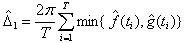
For circular distributions, Dhat2 is equivalent to Dhat1, and Dhat3 is inapplicable.
Dhat4 and Dhat5 use vectors of densities estimated at the times of the observations of the species, x and y:


where n, m are the sample sizes and I is the indicator function (1 if the condition is true, 0 otherwise).
Dhat5 simply checks which curve is higher at each point; even tiny changes in the data can result in large, discontinuous changes in Dhat5, and it can take values > 1. Don't use Dhat5.
Comparing curves at times of actual observations works well if there are enough observations of each species. Simulations show that Dhat4 is best when the smallest sample has at least 50 observations. Dhat1 compares curves at n.grid equally spaced points, and is best for small samples.
Value
A named numeric vector of overlap coefficient estimates. When
type = "all" it has three elements, Dhat1, Dhat4 and Dhat5;
otherwise it has a single element named after the requested estimator. Each
value lies between 0 (no overlap) and 1 (identical activity distributions).
Examples
set.seed(42)
species_A <- runif(100, 1.2, 2 * pi)
species_B <- runif(100, 0.23, 2 * pi)
ct_overlap_estimates(species_A, species_B)
ct_overlap_estimates(species_A, species_B, type = "Dhat4")
Estimate overlap coefficients for multiple species
Description
This function calculates pairwise overlap coefficients for activity patterns of multiple species using their time data.
Usage
ct_overlap_matrix(
  data,
  species_column,
  time_column,
  convert_time = FALSE,
  format = "%H:%M:%S",
  fill_na = NULL,
  ...
)
Arguments
data |
A |
species_column |
A column in |
time_column |
A column in |
convert_time |
Logical. If |
format |
A character string specifying the time format (e.g., |
fill_na |
Optional. A numeric value used to fill |
... |
Additional arguments passed to |
Details
The function calculates pairwise overlap coefficients for all species in the dataset.
The overlap coefficients are estimated using the overlap package:
For species pairs with sample sizes of at least 50 observations each, the
Dhat4estimator is used.For smaller sample sizes, the
Dhat1estimator is used (Schmid & Schmidt, 2006).
Value
A square matrix of pairwise overlap coefficients, where rows and columns represent species.
References
Schmid & Schmidt (2006) Nonparametric estimation of the coefficient of overlapping - theory and empirical application, Computational Statistics and Data Analysis, 50:1583-1596.
See Also
overlap::overlapEst() for overlap coefficient estimation.
Examples
# Example dataset
data <- data.frame(
  species = c("SpeciesA", "SpeciesA", "SpeciesB", "SpeciesB"),
  time = c("10:30:00", "11:45:00", "22:15:00", "23:30:00")
)

# Calculate overlap coefficients with time conversion
overlap_matrix <- ct_overlap_matrix(
  data = data,
  species_column = species,
  time_column = time,
  convert_time = TRUE,
  format = "%H:%M:%S"
)

# Fill missing values in the matrix with 0
overlap_matrix_filled <- ct_overlap_matrix(
  data = data,
  species_column = species,
  time_column = time,
  convert_time = TRUE,
  fill_na = 0
)
Plot a calendar heatmap of daily camera trap activity
Description
Visualises a year of camera-trap records as a calendar heatmap. Tiles are shaded by the number of records per day, or by the summed value of a chosen column. A count distribution can optionally be fitted to the daily values and used for the shading.
Usage
ct_plot_calendar(
  data,
  datetime,
  format = NULL,
  size_column = NULL,
  only_month = NULL,
  fit_distribution = FALSE,
  abbreviate_month_name = FALSE,
  month_name = NULL,
  day_name = NULL,
  number_of_column = 4,
  low = NULL,
  high = NULL,
  palette = NULL,
  na_value = "grey95",
  show_day_number = TRUE,
  title = NULL
)
Arguments
data |
A data frame of records, one row per detection. |
datetime |
Column holding the date or date-time of each record. |
format |
Optional date format(s) passed to |
size_column |
Optional column whose values are summed per day, for example the number of individuals recorded in each detection. If omitted, the number of records (detections) per day is used instead. |
only_month |
Optional integer vector of month numbers (1 to 12) to keep,
for example |
fit_distribution |
Logical. If |
abbreviate_month_name |
Logical. Use three-letter month names. Ignored
when |
month_name |
Optional length-12 character vector of month labels, for localisation. Defaults to the English month names. |
day_name |
Optional length-7 character vector of weekday labels, Monday
first. Defaults to |
number_of_column |
Number of month panels per row. Default |
low, high |
Optional start and end colours for a two-colour gradient
fill. When both are supplied they override |
palette |
Optional fill palette. Either a single viridis option letter
(for example |
na_value |
Fill colour for days with no records. Default |
show_day_number |
Logical. Print the day number inside each tile.
Default |
title |
Optional plot title. Generated automatically when |
Details
With fit_distribution = FALSE the calendar is an activity map: tiles are
shaded by the records per day (or the summed size_column), so busier days
are brighter.
With fit_distribution = TRUE the calendar is instead a typicality map. A
single distribution is fitted to the whole displayed period, and each tile is
shaded by the fitted probability of that day's count. Because most days have
no detection, the count of zero is the most probable value, so empty days
receive the highest density and the brightest colour, while the rarer busy
days appear darker. The map highlights how typical or
unusual each day is under the model, rather than how much activity occurred.
Use fit_distribution = FALSE if you want activity intensity instead.
Value
A ggplot2::ggplot object.
See Also
ct_fit_distribution(), ct_plot_camtrap_activity()
Examples
library(dplyr)
data(ACBR)

# The calendar covers one year at a time, so keep a single year.
d2024 <- ACBR$acbr_data %>%
  # Filter to independent (10min separated) detections
  ct_independence(species_column = species,
                  datetime = datetime,
                  format = "%Y-%m-%d %H:%M:%S",
                  threshold = 10*60
  ) %>%
  # Select data for 2025 year
  filter(lubridate::year(datetime) == 2025)

ct_plot_calendar(d2024, datetime = datetime,
                 size_column = count,
                 low = "gray", high = "red"
)
#'
Plot camera trap activity over time
Description
Visualizes the activity history of camera trap deployments to show periods of data capture. It also optionally highlights periods of inactivity (break/gap).
Usage
ct_plot_camtrap_activity(
  data,
  deployment_column,
  datetime_column,
  threshold = 5,
  time_unit = "days",
  format = NULL,
  activity_style = list(linewidth = 0.8, color = "steelblue", alpha = 0.7, linetype = 1,
    label = "Active period"),
  break_style = list(linewidth = 0.8, color = "#c90026", alpha = 0.9, linetype = 1, label
    = "Break period"),
  show_gaps = TRUE,
  ylabel_format = "%Y-%m-%d",
  ybreak = paste(1, time_unit),
  legend_title = "Activity"
)
Arguments
data |
A data frame containing the datetime column. |
deployment_column |
Column name (unquoted) that identifies the deployment or camera ID. |
datetime_column |
The datetime column. |
threshold |
A numeric value indicating the minimum gap to be considered a break (default is 10). |
time_unit |
The unit for the threshold. Supported values include "secs", "mins", "hours", "days", and "weeks". |
format |
Optional. A character string specifying the datetime format, passed to |
activity_style |
A list controlling the appearance of active periods. Can include:
|
break_style |
A list controlling the appearance of gaps/inactive periods. Can include:
|
show_gaps |
Logical. If |
ylabel_format |
Character. Format for y-axis date-time labels. Default is |
ybreak |
Character. Spacing for y-axis breaks, e.g., |
legend_title |
Character. Title of the colour legend that distinguishes
active periods from breaks (default |
Value
A ggplot2 object showing periods of activity (and optionally gaps)
for each deployment. Active periods and breaks are mapped to colour, so a
legend is drawn (blue for active periods, red for breaks by default). Because
the return value is a standard ggplot object, it can be customised further
with the usual + syntax (for example + ggplot2::labs() or
+ ggplot2::theme()).
Examples
# Load example data and filter for one project phase
data(penessoulou)

camtrap_data <- penessoulou %>%
  dplyr::filter(project == "Last")

# Plot with default styles (a legend distinguishes active periods from breaks)
ct_plot_camtrap_activity(
  data = camtrap_data,
  deployment_column = camera,
  datetime_column = datetimes,
  threshold = 7,
  time_unit = "days"
)

# Customise the colours, the legend labels and the legend title
ct_plot_camtrap_activity(
  data = camtrap_data,
  deployment_column = camera,
  datetime_column = "datetimes",
  threshold = 15,
  time_unit = "days",
  ybreak = "3 days",
  activity_style = list(linewidth = 1.1, color = "gray10", label = "Recording"),
  break_style = list(color = "orange", label = "Gap"),
  legend_title = "Camera status"
)

# The result is a ggplot, so it can be extended with the usual + syntax
ct_plot_camtrap_activity(
  data = camtrap_data,
  deployment_column = camera,
  datetime_column = datetimes,
  threshold = 7,
  time_unit = "days"
) +
  ggplot2::labs(title = "Camera activity") +
  ggplot2::theme(legend.position = "bottom")
Plot species' activity patterns
Description
This function visualizes species' activity patterns based on time-of-day data. It uses kernel density estimation to estimate activity density.
Usage
ct_plot_density(
  time_of_day,
  xscale = 24,
  xcenter = c("noon", "midnight"),
  n_grid = 128,
  kmax = 3,
  adjust = 1,
  rug = FALSE,
  line_type = 2,
  line_color = "gray10",
  line_width = 1,
  rug_lentgh = 0.018,
  rug_color = "gray30",
  extend = "lightgrey",
  extend_alpha = 0.8,
  ...
)
Arguments
time_of_day |
A numeric vector of time-of-day observations (in radians, 0 to |
xscale |
A numeric value to scale the x-axis. Default is 24 for representing time in hours. |
xcenter |
A string indicating the center of the x-axis. Options are |
n_grid |
An integer specifying the number of grid points for density estimation. Default is 128. |
kmax |
An integer indicating the maximum number of modes allowed in the activity pattern. Default is 3. |
adjust |
A numeric value to adjust the bandwidth of the kernel density estimation. Default is 1. |
rug |
A logical value indicating whether to include a rug plot of the observations. Default is |
line_type |
A numeric specifying the line types. Default is 2. |
line_color |
A string specifying the colors of the density lines. Default is "gray10". |
line_width |
A numeric value specifying the line width. Default is 1. |
rug_lentgh |
A numeric value specifying the length of the rug ticks. Default is |
rug_color |
A string specifying the color of the rug ticks. Default is |
extend |
A string specifying the color of the extended area beyond the activity period. Default is |
extend_alpha |
A numeric value (0 to 1) for the transparency of the extended area. Default is |
... |
Additional arguments passed to the |
Value
A ggplot object representing the activity density curves of the species.
Examples
 # Generate random data for two species
 set.seed(42)
 A <- runif(100, 0, 2 * pi)

 # Plot overlap with default settings
 ct_plot_density(A)
 # Customize plot with specific colors and line types
 ct_plot_density(A, line_color = "gray10", line_width = 0.8,
                 xcenter = "midnight", rug = TRUE,
                 rug_color = 'red', extend_alpha = 0)
Plot diversity interploation and extrapolation
Description
plot sample-size-based and coverage-based rarefaction/extrapolation curves along with a bridging sample completeness curve
Usage
ct_plot_inext(
  inext_object,
  type = 1,
  se = TRUE,
  facet_var = "None",
  color_var = "Assemblage",
  grey = FALSE
)
Arguments
inext_object |
an object as outputed by |
type |
three types of plots:
|
se |
a logical variable to display confidence interval around the estimated sampling curve. |
facet_var |
create a separate plot for each value of a specified variable:
|
color_var |
create curves in different colors for values of a specified variable:
|
grey |
a logical variable to display grey and white ggplot2 theme |
Value
a ggplot2 object
Examples
if (requireNamespace("iNEXT", quietly = TRUE)) {
## Import example data
data(penessoulou)
camdata1 <- penessoulou %>%
  dplyr::filter(project == "Last") %>%
  dplyr::mutate(site = "pene") %>%
  # remove consecutive entry of the same species at the same location within 60s
  ct_independence(species_column = species,
                  site_column = camera,
                  datetime = datetimes,
                  threshold = 60, format = "%Y-%m-%d %H:%M:%S"
                  )
head(camdata1)

# Prepare sampling data (camera-day)
camday <- ct_camera_day(
  data = camdata1,
  deployment_column = camera,
  datetime_column = datetime,
  species_column = species,
  size_column = number
)

# RAREFACTION/EXTRAPOLATION
int_ext <- ct_inext(data = camday,
                    diversity_order = c(0, 1, 2),
                    species_column = species,
                    site_column = sampling_unit,
                    size_column = number,
                    n_bootstrap = 50)
int_ext

# plot with curves colored by order
ct_plot_inext(int_ext, type = 1, color_var = "Order.q")

# plot with curves faceted by order
ct_plot_inext(int_ext, type = 1, facet_var = "Order.q")
 }
Plot overlap between two species' activity patterns
Description
This function visualizes the temporal overlap between two species' activity patterns based on time-of-day data. It uses kernel density estimation to estimate activity densities and highlights areas of overlap between the two species.
Usage
ct_plot_overlap(
  A,
  B,
  xscale = 24,
  xcenter = c("noon", "midnight"),
  n_grid = 128,
  kmax = 3,
  adjust = 1,
  rug = FALSE,
  overlap_color = "gray40",
  overlap_alpha = 0.8,
  line_type = c(1, 2),
  line_color = c("gray10", "gray0"),
  line_width = c(1, 1),
  overlap_only = FALSE,
  rug_lentgh = 0.018,
  rug_color = "gray30",
  extend = "lightgrey",
  extend_alpha = 0.8,
  ...
)
Arguments
A |
A numeric vector of time-of-day observations (in radians, 0 to |
B |
A numeric vector of time-of-day observations (in radians, 0 to |
xscale |
A numeric value to scale the x-axis. Default is 24 for representing time in hours. |
xcenter |
A string indicating the center of the x-axis. Options are |
n_grid |
An integer specifying the number of grid points for density estimation. Default is 128. |
kmax |
An integer indicating the maximum number of modes allowed in the activity pattern. Default is 3. |
adjust |
A numeric value to adjust the bandwidth of the kernel density estimation. Default is 1. |
rug |
A logical value indicating whether to include a rug plot of the observations. Default is |
overlap_color |
A string specifying the color of the overlap area. Default is |
overlap_alpha |
A numeric value (0 to 1) for the transparency of the overlap area. Default is 0.8. |
line_type |
A vector of integers specifying the line types for species A and B density lines. Default is |
line_color |
A vector of strings specifying the colors of the density lines for species A and B. Default is |
line_width |
A vector of numeric values specifying the line widths for species A and B density lines. Default is |
overlap_only |
A logical value indicating whether to plot only the overlap region without individual density lines. Default is |
rug_lentgh |
A numeric value specifying the length of the rug ticks. Default is 0.018 (in normalized plot coordinates). |
rug_color |
A string specifying the color of the rug ticks. Default is |
extend |
A string specifying the color of the extended area beyond the activity period. Default is |
extend_alpha |
A numeric value (0 to 1) for the transparency of the extended area. Default is 0.8. |
... |
Additional arguments passed to the |
Value
A ggplot object representing the activity density curves and overlap between the two species.
If overlap_only = TRUE, only the overlap region is displayed.
Examples
  # Generate random data for two species
  set.seed(42)
  species_A <- runif(100, 0, 2 * pi)
  species_B <- runif(100, 0, 2 * pi)

  # Plot overlap with default settings
  ct_plot_overlap(A = species_A, B = species_B)

  # Customize plot with specific colors and line types
  ct_plot_overlap(A = species_A, B = species_B, overlap_color = "blue",
  line_color = c("red", "green"))

  # Include rug plots and change transparency
  ct_plot_overlap(A = species_A, B = species_B, rug = TRUE,
  overlap_alpha = 0.5)
Plot overlap coefficient matrix
Description
Visualizes an overlap coefficient matrix.
Usage
ct_plot_overlap_coef(
  data,
  side = c("lower", "upper"),
  show = c("shape", "value"),
  shape_type = 21,
  shape_size = 0.5,
  text_size = 6,
  text_font = NA,
  excludes = NULL,
  color_scale = "gray3",
  ...
)
Arguments
data |
A square matrix (e.g |
side |
A character string indicating which triangle of the matrix to display. Options are "lower" (default) or "upper". |
show |
A character string specifying whether to display "shape" (default) or "value" in the plot. |
shape_type |
Numeric value specifying the type of shape to use in the plot. Defaults to 21 (circle). |
shape_size |
Numeric value controlling the stroke size of the shapes. Defaults to 0.5. |
text_size |
Numeric value specifying the size of the text when |
text_font |
Character string specifying the font family to use for text labels.
Defaults to |
excludes |
A vector of numeric values to exclude from the plot. Defaults to |
color_scale |
A character string or vector of colors to define the gradient color scale. Defaults to "gray3". |
... |
Additional arguments passed to the |
Value
A ggplot object representing the overlap coefficient matrix visualization.
Examples
library(ggplot2)
# Example overlap coefficient matrix
overlap_matrix <- matrix(c(1, 0.8, 0.7, 0.8, 1, 0.9, 0.7, 0.9, 1), ncol = 3)
colnames(overlap_matrix) <- rownames(overlap_matrix) <- c("A", "B", "C")

# Plot lower triangle with shapes
ct_plot_overlap_coef(overlap_matrix, side = "lower", show = "shape")

# Plot upper triangle with values
ct_plot_overlap_coef(overlap_matrix, side = "upper", show = "value")
Plot a 24-hour rose diagram of daily activity
Description
This function generates a rose diagram (circular bar plot) to visualize daily activity patterns over a 24-hour period. Each bar represents either the absolute or relative frequency of observations within hourly intervals. The plot also includes a segment indicating the mean activity time, and an optional segment showing the 95% confidence interval of the activity period.
Usage
ct_plot_rose_diagram(
  data = NULL,
  times,
  frequencies = "absolute",
  hide_lebels = FALSE,
  label_position = NULL,
  label_style = list(),
  time_range = 1,
  ci_segment = TRUE,
  mean_segment = TRUE,
  ring = TRUE,
  color = "gray20",
  fill = color,
  ci_style = list(),
  mean_style = list(),
  start = -0.12,
  width = NULL
)
Arguments
data |
A data frame containing the time values. If |
times |
A numeric vector of time values (in radians) or a column name from |
frequencies |
Character. Use |
hide_lebels |
Logical. If |
label_position |
Numeric. Controls vertical position of the frequency value labels (if shown). |
label_style |
A list of styles for labels. Accepts |
time_range |
Numeric. Width of the time bins in hours. Default is |
ci_segment |
Logical or numeric. If |
mean_segment |
Logical. If |
ring |
Logical or numeric vector. If |
color |
Color of the bar border and segments. Default is |
fill |
Fill color of the bars. Default is the same as |
ci_style |
A list of styles for the confidence interval segment. Accepts |
mean_style |
A list of styles for the mean segment. Accepts |
start |
Numeric. The angle (in radians) where the polar plot starts. Default is |
width |
Numeric. Width of each bar. Default is |
Value
A ggplot object representing the rose diagram.
Examples
set.seed(129)
library(dplyr)
library(ggplot2)

rf <- runif(123, 0, max = 6)

ct_plot_rose_diagram(data = NULL,
                     times = rf,
                     frequencies = "relative",
                     label_style = list(size = 4, color = 'red'),
                     label_position = 11,
                     time_range = 1,
                     mean_segment = TRUE,
                     ci_segment = 1,
                     ring = c(-5, 12),
                     color = 'gray20',
                     mean_style = list(linetype = 1, linewidth = .5, color = 'red'),
                     ci_style = list(linetype = 1, linewidth = .5, color = 'black')
)
Read a delimited file into a tibble
Description
The ct_read function reads a delimited text file.
It automatically detects the delimiter if not specified and provides an easy-to-use
interface for importing data with additional customization options.
Usage
ct_read(file_path, header = TRUE, sep, ...)
Arguments
file_path |
A string specifying the path to the file to be read. |
header |
A logical value indicating whether the file contains a header row. Defaults to |
sep |
The field separator character. If not provided, the function automatically detects the separator. |
... |
Additional arguments passed to the |
Value
A tibble containing the data from the specified file.
Read Image Metadata
Description
Extracts metadata from image files using ExifTool and returns the results as a tibble.
Usage
ct_read_metadata(
  path,
  tags = NULL,
  recursive = FALSE,
  parse_hs = FALSE,
  args = NULL,
  exiftool_path = NULL
)
Arguments
path |
Character vector of image file paths or a directory path. |
tags |
Character vector of tag names to extract. Use:
|
recursive |
Logical. If |
parse_hs |
Logical. If |
args |
Character vector of additional arguments passed directly to
ExifTool (e.g., |
exiftool_path |
Character. Path to the ExifTool executable. If
|
Details
By default, all available tags are returned. You can limit the output to a predefined set of tags or provide a custom list of tag names.
This function calls ExifTool with CSV output enabled and numeric values
returned where applicable. When parse_hs = TRUE, the
HierarchicalSubject field is split into structured columns.
Value
A tibble where each row represents one image file and each column represents a metadata field.
See Also
-
ct_get_hs()to retrieve hierarchical subjects -
ct_create_hs()to add hierarchical subjects -
ct_remove_hs()to remove hierarchical subjects
Examples
## Not run:
# Example image path
image_path <- file.path(system.file("img", package = "ct"), "large.jpeg")

# Extract all metadata
ct_read_metadata(path = image_path)

# Extract a predefined standard set of metadata
ct_read_metadata(path = image_path, tags = "standard")

# Extract custom tags
ct_read_metadata(path = image_path,
                 tags = c("DateTimeOriginal", "GPSLatitude", "GPSLongitude"))

# Parse hierarchical subject fields into columns
ct_read_metadata(path = image_path,
                 tags = "standard",
                 parse_hs = TRUE)

## End(Not run)
Remove hierarchical subject (hs) values from image metadata
Description
Removes specific hierarchical subjects or clears the entire HierarchicalSubject field from image metadata using ExifTool. Can remove one or multiple specific parent|child hierarchies, or clear all hierarchical subjects at once.
This function supports processing individual files or entire directories (with optional recursion), applying the removal to all supported image files found.
Usage
ct_remove_hs(
  path,
  hierarchy = NULL,
  recursive = FALSE,
  intern = TRUE,
  quiet = TRUE,
  ...
)
Arguments
path |
A character string specifying the full path to an image file or directory. If a directory is provided, hierarchical subjects will be removed from all supported image files in that directory. |
hierarchy |
A named character vector specifying hierarchies to remove.
Names represent parent categories, values represent child categories.
Example: |
recursive |
Logical. If |
intern |
Logical. If |
quiet |
Logical. If |
... |
Additional arguments passed to |
Details
When removing specific hierarchies from a single file, the function validates that they exist before attempting removal. If the last hierarchy is removed, the entire HierarchicalSubject field is cleared from the metadata. The function handles multiple hierarchies in a single call.
When processing directories, the function applies the removal to all supported
image files found. Use recursive = TRUE to include subdirectories. Note that
validation of existing hierarchies is only performed for single files.
Value
Invisibly returns TRUE on success, FALSE if specified hierarchy
doesn't exist. Displays informative messages about the operation. Called
primarily for side effects (modifying image metadata).
See Also
-
ct_get_hs()to retrieve hierarchical subjects -
ct_create_hs()to add hierarchical subjects -
ct_read_metadata()to read image metadata
Examples
## Not run:
# Path to example image
image_path <- file.path(system.file("img", package = "ct"), "large.jpeg")

# Add some hierarchical subjects
ct_create_hs(image_path, c("Species" = "Vulture", "Location" = "Africa"))
ct_get_hs(image_path)

# Remove a specific hierarchy
ct_remove_hs(image_path, hierarchy = c("Species" = "Vulture"))
ct_get_hs(image_path) # Only "Location|Africa" remains

# Remove multiple hierarchies at once
ct_create_hs(image_path, c("Species" = "Eagle", "Status" = "Endangered"))
ct_remove_hs(
  image_path,
  hierarchy = c("Species" = "Eagle", "Status" = "Endangered")
)

# Remove all hierarchical subjects
ct_remove_hs(image_path, hierarchy = NULL)
ct_get_hs(image_path) # Returns NULL

# Attempting to remove non-existent hierarchy
ct_remove_hs(image_path, hierarchy = c("Species" = "NonExistent"))

# Remove all hierarchical subjects from all images in a directory
image_dir <- system.file("img", package = "ct")
ct_remove_hs(path = image_dir, recursive = FALSE)

# Remove recursively from directory and subdirectories
ct_remove_hs(path = image_dir, recursive = TRUE)

# Remove specific hierarchy from all images in a directory
ct_remove_hs(
  path = image_dir,
  hierarchy = c("Species" = "Vulture"),
  recursive = TRUE
)

## End(Not run)
Prepare activity (time-of-day) data for REST
Description
Keeps independent detections of each species and converts their time of day to radians for circular activity modelling.
Usage
ct_rest_activity(
  detection_data,
  station_column = "Station",
  species_column = "Species",
  datetime_column = "DateTime",
  independence_minutes = 30
)
Arguments
detection_data |
A data frame with one row per detection. |
station_column, datetime_column |
Columns for the station ID and datetime
in |
species_column |
Column for species in |
independence_minutes |
Minimum gap (minutes) between successive detections at a station for them to count as independent. |
Value
A tibble with columns Species, Station, time (radians).
Examples
data(rest_detection)

activity <- ct_rest_activity(rest_detection, independence_minutes = 30)
head(activity)
Add camera-trapping effort (days) to formatted station data
Description
Effort is approximated as the span between the first and last detection. When
term_col is given, effort is computed per survey term and summed per station
so inactive gaps between terms are not counted.
Usage
ct_rest_effort(
  detection_data,
  station_data,
  station_column = "Station",
  datetime_column = "DateTime",
  term_column = NULL,
  plot = FALSE
)
Arguments
detection_data |
A data frame with one row per detection. |
station_data |
A data frame from |
station_column, datetime_column |
Columns for the station ID and datetime
in |
term_column |
Optional column identifying survey terms;
|
plot |
If |
Value
station_data with an added Effort column (days). Stations with no
or zero effort are dropped with a warning.
Examples
data(rest_detection)
data(rest_station)

stations <- ct_rest_passes(rest_detection, rest_station, model = "REST")
ct_rest_effort(rest_detection, stations)
Aggregate the number of animal passes per station for REST / RAD-REST
Description
Aggregate the number of animal passes per station for REST / RAD-REST
Usage
ct_rest_passes(
  detection_data,
  station_data,
  station_column = "Station",
  species_column = "Species",
  passes_column = "y",
  model = c("REST", "RAD-REST")
)
Arguments
detection_data |
A data frame with one row per video / detection. |
station_data |
A data frame with one row per camera station. |
station_column, species_column |
Columns giving the station ID and species
in |
passes_column |
Column holding the number of passes per video. |
model |
Either |
Value
A tibble with one row per station x species, ready for ct_rest_effort().
Examples
data(rest_detection)
data(rest_station)

# Original REST: total passes (Y) per station
ct_rest_passes(rest_detection, rest_station, model = "REST")

# RAD-REST: videos split by number of passes (y_0, y_1, ...)
ct_rest_passes(rest_detection, rest_station, model = "RAD-REST")
Choose a staying-time distribution for REST by WAIC
Description
Fits the REST staying-time survival sub-model under one or more candidate
distributions (and, optionally, covariate combinations) and ranks them by
WAIC, with a Bayesian p-value as a goodness-of-fit check. Use the winning
stay_distribution in ct_fit_rest().
Usage
ct_rest_select_stay(
  stay_data,
  species,
  stay_formula = Stay ~ 1,
  stay_distribution = c("lognormal", "gamma", "weibull", "exponential"),
  stay_random_effect = NULL,
  compare_models = FALSE,
  iterations = 5000,
  burnin = 1000,
  thin = 4,
  chains = 3,
  cores = 3,
  quiet = FALSE
)
Arguments
stay_data |
Staying-time data from |
species |
Single species name to analyse. |
stay_formula |
Staying-time formula, e.g. |
stay_distribution |
One or more of |
stay_random_effect |
Optional column in |
compare_models |
If |
iterations, burnin, thin, chains, cores |
MCMC settings. |
quiet |
If |
Value
An object of class ct_rest_stay with a waic ranking tibble, a
summary of the mean staying time for the best model, and its samples.
See Also
Examples
data(rest_detection)
data(rest_station)

stay <- ct_rest_stay(rest_detection, rest_station)

## Not run:
# Compare candidate staying-time distributions by WAIC (requires 'nimble')
ct_rest_select_stay(
  stay, species = "Red duiker",
  stay_distribution = c("lognormal", "gamma", "weibull"),
  iterations = 3000, burnin = 1000, chains = 2, cores = 2
)

## End(Not run)
Prepare staying-time data for REST
Description
Selects and standardises the staying-time and censoring columns from a detection table and attaches per-station covariates.
Usage
ct_rest_stay(
  detection_data,
  station_data,
  station_column = "Station",
  species_column = "Species",
  stay_column = "Stay",
  censor_column = "Cens"
)
Arguments
detection_data |
A data frame with one row per video / detection. |
station_data |
A data frame with one row per camera station. |
station_column, species_column |
Columns giving the station ID and species
in |
stay_column |
Column holding the staying time in seconds. |
censor_column |
Column holding the censoring flag (1 = censored, 0 = fully observed). |
Value
A tibble with columns Station, Species, Stay, Cens plus any
station covariates, ready for ct_fit_rest().
Examples
data(rest_detection)
data(rest_station)

# Column names can be strings, bare names, or positions:
stay <- ct_rest_stay(rest_detection, rest_station, stay_column = Stay)
head(stay)
Model selection for Distance Sampling detection functions
Description
Implements a two-step model selection procedure for distance sampling detection functions following the approach of Howe et al (2019).
Usage
ct_select_model(models, chat = NULL, k = 2)
Arguments
models |
A list of fitted detection function models (objects returned by
|
chat |
Optional numeric value of overdispersion ( |
k |
Numeric. The penalty term used in QAIC (default is |
Details
Step 1:
Within each key function family (e.g., half-normal, hazard-rate), models are compared
using the quasi-Akaike Information Criterion (QAIC). Overdispersion (\hat{c})
is estimated if not provided. The best model per key function family is identified as
the one with the lowest QAIC.
Step 2:
The best models from each key function family are compared using overall goodness-of-fit
statistics based on chi-squared divided by degrees of freedom (\chi^2 / df).
The model with the lowest \chi^2 / df is selected as the final detection function model.
Value
A named list with the following elements:
-
QAIC: A tibble summarizing QAIC results for each model within key function families. -
Best QAIC models: A subset of models, one per key function, that minimize QAIC. -
Chiq2: A tibble comparing the best models by chi-squared goodness-of-fit criteria. -
Final model: The selected detection function model with the lowest chi-squared/df.
References
Howe, E. J., Buckland, S. T., Després-Einspenner, M., & Kühl, H. S. (2019). Model selection with overdispersed distance sampling data. Methods in Ecology and Evolution, 10(1), 38-47. doi:10.1111/2041-210X.13082
See Also
Examples
library(Distance)
library(dplyr)

data("duiker")
duiker_data <- duikers$DaytimeDistances %>%
  dplyr::slice_sample(prop = .3) # sample 30% of rows
truncation <- list(left = 2, right = 15) # Keep only distance between 2-15 m

# fit hazard-rate key models
w3_hr0 <- ds(duiker_data, transect = "point", key = "hr", adjustment = NULL,
             truncation = truncation)
w3_hr1 <- ds(duiker_data, transect = "point", key = "hr", adjustment = "cos",
             order = 2, truncation = truncation)
w3_hr2 <- ds(duiker_data, transect = "point", key = "hr", adjustment = "cos",
             order = c(2, 4), truncation = truncation)
# fit half-normal key models
w3_hn0 <- ds(duiker_data, transect = "point", key = "hn", adjustment = NULL,
             truncation = truncation)
w3_hn1 <- ds(duiker_data, transect = "point", key = "hn", adjustment = "cos",
             order = 2, truncation = truncation)
w3_hn2 <- ds(duiker_data, transect = "point", key = "hn", adjustment = "cos",
             order = c(2, 4), truncation = truncation)
# fit uniform key models
w3_u0 <- ds(duiker_data, transect = "point", key = "unif", adjustment = NULL,
            truncation = truncation)
w3_u1 <- ds(duiker_data, transect = "point", key = "unif", adjustment = "cos",
            order = 2, truncation = truncation)
w3_u2 <- ds(duiker_data, transect = "point", key = "unif", adjustment = "cos",
            order = c(2, 4), truncation = truncation)

# Create model list
model_list <- list(w3_hn0, w3_hn1, w3_hn2,
                   w3_hr0, w3_hr1, w3_hr2,
                   w3_u0, w3_u1, w3_u2)

# Compute model QAICs
ct_QAIC(list(w3_hr0, w3_hr1, w3_hr2)) # All key functions must be the same
ct_QAIC(list(w3_hn0, w3_hn1, w3_hn2)) # All key functions must be the same

# Compute Chi-squared Goodness-of-fit
ct_chi2_select(list(w3_hn0, w3_hr0, w3_u0)) # All key functions must be different
ct_chi2_select(list(w3_hn2, w3_hr1, w3_u0)) # All key functions must be different

# Two-step model selection
ct_select_model(model_list)
Transform time to solar time anchored to sunrise and sunset
Description
This function converts local time to solar time based on the sunrise and sunset times for a given location. Solar time is a timekeeping system where the day is defined by the position of the sun in the sky, with sunrise marking the start of the day and sunset marking the end.
Usage
ct_solartime(
  data = NULL,
  date,
  longitude,
  latitude,
  crs = NULL,
  format,
  time_zone,
  ...
)
Arguments
data |
A data frame containing the date, longitude, and latitude columns.
If |
date |
A vector of date-time values or a column name in |
longitude |
A numeric vector or a column name in |
latitude |
A numeric vector or a column name in |
crs |
A coordinate reference system (CRS) string or object specifying the
current CRS of the input coordinates. If provided, the function will transform
the coordinates to longitude and latitude (WGS84). This is useful when the input
coordinates are in a projected system (e.g., UTM). Default is |
format |
character string giving a date-time format as used by |
time_zone |
A numeric vector representing the time zone offset(s) from UTC
(in hours). If |
... |
Additional arguments passed to |
Details
The function calculates solar time by first determining the sunrise and sunset times for the given location(s) and date(s). It then uses these times to anchor the solar time calculation. The solar time is computed by transforming the local clock time based on the position of the sun in the sky.
If data is provided, the function will process each unique location in the
data and return a tibble with the solar time for each date-time value. If data
is NULL, the function will process the date, longitude, and latitude
parameters directly.
Value
A tibble with the following columns:
-
input: The original date-time values. -
clock: The local clock time. -
solar: The calculated solar time.
If data is provided, the tibble will also include the longitude and latitude columns.
References
Rowcliffe, M. (2023). activity: Animal Activity Statistics. R package version 1.3.4. https://CRAN.R-project.org/package=activity
Examples
library(dplyr)
data(penessoulou)

cam_data <- penessoulou %>%
  dplyr::filter(project == "Last") %>%
 dplyr::filter(species == "Erythrocebus patas") %>%
 # Select independent events based on a given threshold
 ct::ct_independence(species_column = species,
                          datetime = datetimes, threshold = 60*5, # 5 minutes
                          format = "%Y-%m-%d %H:%M:%S"
                          ) %>%
 # Transform Time to Solar Time
 ct_solartime(data = ., date = datetime, longitude = longitude, latitude = latitude,
               crs = "EPSG:32631", time_zone = 1)
Estimate species spatial coverage from camera trap detections
Description
Estimates spatial coverage
a species from camera-trap detection data using a kernel density approach.
The kernel bandwidth \hat{\sigma} is estimated from the
spatial spread of detection sites via Silverman's reference bandwidth rule
(Silverman 1986).
Usage
ct_spatial_coverage(
  data,
  site_column,
  longitude,
  latitude,
  crs = c(4326, NULL),
  study_area = NULL,
  mask = NULL,
  resolution,
  isopleth = 0.95,
  n_boot = 200
)
Arguments
data |
A data frame of species detection records. |
site_column |
Column name of the camera-trap site identifier. |
longitude |
Column name of site longitude (or UTM easting). |
latitude |
Column name of site latitude (or UTM northing). |
crs |
A vector of length two specifying the coordinate reference systems:
|
study_area |
Optional |
mask |
Optional |
resolution |
Numeric. Side length of one grid cell in the units of the active CRS (metres if projected). |
isopleth |
Numeric in |
n_boot |
Integer. Bootstrap resamples for the standard error of
|
Details
The term home range is typically associated with dynamic movement data, such as those recorded by radio-tracking or GPS devices, which provide continuous or near-continuous tracking of an individual animal's movements. Since camera traps are static and only capture presence/absence or activity within their specific locations, the concept of home range might not fully apply.
Method
Each camera station where the species was detected contributes equally (binary detection). A Gaussian kernel is centred at each detection site and the average surface is computed:
  \hat{f}(\mathbf{x}) =
    \frac{1}{n} \sum_{i=1}^{n}
    \exp\!\left(-\frac{\|\mathbf{x} - \mathbf{x}_i\|^2}{2\,\hat{\sigma}^2}\right)
Bandwidth estimation
The bandwidth \hat{\sigma} is the reference bandwidth (Silverman
1986, eq. 4.14, extended to 2-D):
\hat{\sigma} = \sqrt{\hat{\sigma}_x \, \hat{\sigma}_y} \; n^{-1/6}
where \hat{\sigma}_x and \hat{\sigma}_y are the standard
deviations of the detection-site coordinates and n is the number of
detection sites. This is the asymptotically MISE-optimal bandwidth under a
bivariate normal reference distribution. It shrinks with more sites and widens
when detections are spatially dispersed.
The standard error of \hat{\sigma} is obtained by nonparametric
bootstrap: sites are resampled with replacement n_boot times and
\hat{\sigma} recomputed each time; the SE is the standard deviation
of those bootstrap estimates, and the 95 % CI is their 2.5th - 97.5th
percentiles.
Home-range isopleth
Cells are ranked by kernel density (descending). The isopleth isopleth
retains the smallest set of cells whose cumulative density equals
isopleth of the total - the standard minimum-volume contour estimator
(Worton 1989).
Value
A named list with three elements:
Coverage rasterA
SpatRaster(terra) containing the kernel density surface, clipped to theisoplethisopleth, with masked and out-of-isopleth cells set toNA.BandwidthA named numeric vector:
sigma(estimated bandwidth in CRS units),SE(bootstrap SE;NAifn_boot = 0),CI_lowandCI_high(95 % bootstrap CI),n_sites, andisopleth.Coverage statsA one-row tibble: coverage area in km^2,
\hat{\sigma}+/- SE, detection-site count, and isopleth level.
References
Silverman, B. W. (1986). Density Estimation for Statistics and Data Analysis. Chapman and Hall, London.
Worton, B. J. (1989). Kernel methods for estimating the utilization distribution in home-range studies. Ecology, 70(1), 164-168. doi:10.2307/1938423
Examples
library(dplyr)
data(penessoulou)
cam_data <- penessoulou %>%
  dplyr::filter(project == "First") %>%
  dplyr::filter(species == "Erythrocebus patas", number > 0)

spc <- ct_spatial_coverage(
  data = cam_data,
  site_column = camera,
  longitude = longitude,
  latitude = latitude,
  crs = "EPSG:32631",
  resolution = 30 # meter
)

# Plot coverage raster
library(terra)
terra::plot(spc$`Coverage raster`)

## Bandwidth estimate with uncertainty
spc$Bandwidth

## Coverage area summary
spc$`Coverage stats`
Stack a list of data frame
Description
The function takes a list of data frames and stacks them into a single data frame. It ensures that all columns from the input data frames in the list are included in the output, filling in missing columns with NA values where necessary.
Usage
ct_stack_df(df_list)
Arguments
df_list |
list of data frame to be stacked |
Value
data frame
Examples
x <- data.frame(age = 15, fruit = "Apple", weight = 12)
y <- data.frame(age = 51, fruit = "Tomato")
z <- data.frame(age = 26, fruit = "Lemo", weight = 12, height = 45)
alldf <- list(x,y,z)
ct_stack_df(alldf)
Standardize community data matrix
Description
This function standardizes a given data matrix using different methods such as total sum scaling, max normalization, frequency scaling, standardization, presence-absence transformation, chi-square transformation, Hellinger transformation, log transformation, and others.
Usage
ct_standardize(
  data,
  method,
  margin,
  range_global,
  logbase = 2,
  na.rm = FALSE,
  ...
)
Arguments
data |
A numeric matrix or data frame to be standardized. |
method |
A character string specifying the standardization method (see details). Available methods are:
|
margin |
An integer specifying the margin for standardization:
|
range_global |
A matrix specifying the range for standardization
(optional, used with |
logbase |
The base for logarithmic transformation (default is 2). |
na.rm |
Logical. If |
... |
Additional arguments passed to transformation functions. |
Details
The function provides the following standardization methods for community data:
-
"total": Divides by margin total (defaultmargin = 1). -
"max": Divides by margin maximum (defaultmargin = 2). -
"frequency": Divides by margin total and multiplies by the number of non-zero items, ensuring the average of non-zero entries is one (Oksanen 1983; defaultmargin = 2). -
"normalize": Scales data so that the sum of squares along the specified margin equals one (defaultmargin = 1). -
"range": Standardizes values into the range[0,1](defaultmargin = 2). If all values are constant, they will be transformed to 0. -
"rank","rrank":-
"rank"replaces abundance values by their increasing ranks, leaving zeros unchanged. -
"rrank"is similar but uses relative ranks with a maximum of 1 (defaultmargin = 1).
-
-
"standardize": Scalesxto zero mean and unit variance (defaultmargin = 2). -
"pa": Convertsxto presence/absence scale (0/1). -
"chi.square": Divides by row sums and the square root of column sums, then adjusts for the square root of the matrix total (Legendre & Gallagher 2001). When used with Euclidean distance, the distances should be similar to Chi-square distances in correspondence analysis (defaultmargin = 1). -
"hellinger": Computes the square root ofmethod = "total"(Legendre & Gallagher 2001). -
"log": Logarithmic transformation suggested by Anderson et al. (2006):\log_b (x) + 1for
x > 0, wherebis the base of the logarithm. Zeros remain unchanged. Higher bases give less weight to quantities and more to presences. -
"alr": Additive log ratio (ALR) transformation (Aitchison 1986). Reduces skewness and compositional bias. Requires positive values; pseudocounts can be added. The transformation is defined as:alr = [\log(x_1 / x_D), ..., \log(x_{D-1} / x_D)]where the denominator sample
x_Dcan be chosen arbitrarily. -
"clr": Centered log ratio (CLR) transformation (Aitchison 1986). Common in microbial ecology (Gloor et al. 2017). Only supports positive data; pseudocounts can be used to handle zeros. The transformation is defined as:clr = \log(x / g(x)) = \log x - \log g(x)where
xis a single value, andg(x)is the geometric mean ofx. -
"rclr": Robust CLR transformation. Unlike CLR, this method allows zeros without requiring pseudocounts. It divides values by the geometric mean of observed (non-zero) features, preserving zeros (Martino et al. 2019). The transformation is defined as:rclr = \log(x / g(x > 0))where
xis a single value, andg(x > 0)is the geometric mean of sample-wide valuesxthat are positive (x > 0).
Standardization, as contrasted to transformation, means that the entries are transformed relative to other entries.
All methods have a default margin. margin=1 means rows
(sites in a normal data set) and margin=2 means columns (species in a
normal data set).
Command wisconsin is a shortcut to common Wisconsin double
standardization where species (margin=2) are first standardized
by maxima (max) and then sites (margin=1) by
site totals (tot).
Most standardization methods will give nonsense results with
negative data entries that normally should not occur in the community
data. If there are empty sites or species (or constant with
method = "range"), many standardization will change these into
NaN.
Function decobackstand can be used to transform standardized
data back to original. This is not possible for all standardization
and may not be implemented to all cases where it would be
possible. There are round-off errors and back-transformation is not
exact, and it is wise not to overwrite the original data. With
zap=TRUE original zeros should be exact.
Value
A standardized matrix or tibble with attributes specifying the transformation applied.
Note
This function is adapted from the decostand function in the vegan R package,
with modifications to improved handling.
References
Aitchison, J. The Statistical Analysis of Compositional Data (1986). London, UK: Chapman & Hall.
Anderson, M.J., Ellingsen, K.E. & McArdle, B.H. (2006) Multivariate dispersion as a measure of beta diversity. Ecology Letters 9, 683–693.
Egozcue, J.J., Pawlowsky-Glahn, V., Mateu-Figueras, G., Barcel'o-Vidal, C. (2003) Isometric logratio transformations for compositional data analysis. Mathematical Geology 35, 279–300.
Gloor, G.B., Macklaim, J.M., Pawlowsky-Glahn, V. & Egozcue, J.J. (2017) Microbiome Datasets Are Compositional: And This Is Not Optional. Frontiers in Microbiology 8, 2224.
Legendre, P. & Gallagher, E.D. (2001) Ecologically meaningful transformations for ordination of species data. Oecologia 129, 271–280.
Martino, C., Morton, J.T., Marotz, C.A., Thompson, L.R., Tripathi, A., Knight, R. & Zengler, K. (2019) A novel sparse compositional technique reveals microbial perturbations. mSystems 4, 1.
Oksanen, J. (1983) Ordination of boreal heath-like vegetation with principal component analysis, correspondence analysis and multidimensional scaling. Vegetatio 52, 181–189.
Examples
# Example usage with sample data
library(dplyr)
data(penessoulou)

cam_data <- penessoulou %>%
  dplyr::filter(project == "Last")
cam_data <- cam_data %>%
  ct_to_community(site_column = camera, species_column = species,
                  size_column = number, values_fill = 0)

standardized_data <- ct_standardize(data = cam_data[, 2:11], method = "total")
standardized_data
Create activity summary statistics
Description
Calculates summary statistics for camera trap activity periods.
Usage
ct_summarise_camtrap_activity(
  data,
  deployment_column,
  datetime_column,
  threshold = 5,
  time_unit = "days",
  format = NULL
)
Arguments
data |
A data frame containing the datetime column. |
deployment_column |
Character. Column name for deployment identifiers. |
datetime_column |
The datetime column. |
threshold |
A numeric value indicating the minimum gap to be considered a break (default is 10). |
time_unit |
The unit for the threshold. Supported values include "secs", "mins", "hours", "days", and "weeks". |
format |
Optional. A character string specifying the datetime format, passed to |
Value
A tibble with activity summary statistics for each deployment.
Examples
# Get activity summary
library(dplyr)
data(penessoulou)
camtrap_data <- penessoulou %>%
  filter(project == "Last")

ct_summarise_camtrap_activity(data = camtrap_data,
                              deployment_column = "camera",
                              datetime_column = datetimes,
                              threshold = 15,
                              time_unit = "days")
Create a survey design for camera trap deployment
Description
This function designs a survey for deploying camera traps within a specified study area. It supports various sampling methods, including random, regular, and clustered sampling, with options for minimum distance constraints and padding around the study area.
Usage
ct_survey_design(
  study_area,
  method = "random",
  total_site,
  total_cluster,
  type_in = "random",
  min_distance = NULL,
  distance = NULL,
  padding = 10,
  nest_padding = 0,
  set_seed = NULL,
  verbose = TRUE
)
Arguments
study_area |
An |
method |
A character string specifying the sampling method. Options include:
|
total_site |
An integer specifying the number of sites to be sampled per
cluster (for "regular_cluster" and "random_cluster") or the total number of
sites (for "random" and "regular" methods). For the "mask" method, this can
be a single value (applied to all features) or a vector specifying the number
of sites per feature in |
total_cluster |
An integer defining the number of clusters (required for "random_cluster"). |
type_in |
A character string indicating the within-cluster sampling type. Options:
|
min_distance |
A numeric value specifying the minimum allowed distance (in meter) between sampled sites (applied only for the random methods). |
distance |
A numeric vector specifying the distance (x and y spacing in meter) between grid cells for regular sampling methods. If a single value is provided, it is used for both dimensions. |
padding |
A numeric value defining the buffer distance to exclude areas near the edge of the study area. |
nest_padding |
A numeric value defining an additional buffer applied within each cluster or mask feature to avoid placing sites near the edges of those units. |
set_seed |
An optional integer for setting the random seed to ensure reproducibility. |
verbose |
A logical indicating whether to display warnings and messages (default: |
Value
An sf object containing the sampled points within the study area.
Note
The function ensures that the study area has a projected coordinate reference system (CRS) before proceeding. If a geographic CRS is detected, an error is raised.
Examples
library(ggplot2)
# Load example dataset
data("pendjari")

# Transform study area to a projected coordinate system
pendjari_trans <- pendjari %>%
  sf::st_transform(crs = "EPSG:32631")

# Random sampling method with 15 sites, ensuring a minimum distance of 5000 meters between sites
random_sdes <- ct_survey_design(study_area = pendjari_trans, method = "random", verbose = TRUE,
                                total_site = 15, min_distance = 5000, padding = 2000,
                                set_seed = 123)

# Regular sampling method using a grid with cell sizes of 4000m x 6000m
regular_sdes <- ct_survey_design(study_area = pendjari_trans, method = "regular", verbose = TRUE,
                                 distance = c(4000, 6000), padding = 2500, set_seed = 123)

# Random-cluster sampling: 8 clusters, each containing 5 sites, ensuring a
# minimum site distance of 2000 meters
rand_c_sdes <- ct_survey_design(study_area = pendjari_trans,
                                method = "random_cluster", verbose = TRUE,
                                total_cluster = 8, total_site = 5,
                                distance = c(7000, 3000), min_distance = 2000,
                                padding = 2000, nest_padding = 500, set_seed = 123)

# Random-cluster sampling with regularly distributed sites: 22 clusters, each
# with 8 regularly spaced sites
rand_c_reg_sdes <- ct_survey_design(study_area = pendjari_trans,
                                    method = "random_cluster", verbose = TRUE,
                                    total_cluster = 22, total_site = 8, type_in = "regular",
                                    distance = c(6000, 3000),
                                    padding = 1000, nest_padding = 0, set_seed = 123)

# Regular-cluster sampling: Grid with 3 sites per cluster, ensuring a minimum
# distance of 2000 meters between sites
reg_c_sdes <- ct_survey_design(study_area = pendjari_trans,
                               method = "regular_cluster", verbose = TRUE,
                               total_site = 3, distance = c(7000, 6000),
                               min_distance = 2000, padding = 2000, set_seed = 123)

# Regular-cluster sampling with regularly distributed sites within clusters
reg_c_reg_sdes <- ct_survey_design(study_area = pendjari_trans,
                                   method = "regular_cluster", verbose = TRUE,
                                   total_site = 3, distance = c(7000, 6000), type_in = "regular",
                                   padding = 1000, set_seed = 123)
# A plot with
ggplot()+
  geom_sf(data = pendjari_trans)+
  geom_sf(data = reg_c_reg_sdes)

# Mask-based sampling: Sites are sampled within existing features of the study area
mask_sdes <- ct_survey_design(study_area = pendjari_trans,
                              method = "mask", verbose = TRUE,
                              total_site = 13, distance = c(7000, 6000),
                              min_distance = 2000, nest_padding = 2000, set_seed = 123)

# Mask-based sampling with regularly spaced sites per feature
mask_regular_sdes <- ct_survey_design(study_area = pendjari_trans,
                                      method = "mask", verbose = TRUE, type_in = "regular",
                                      total_site = c(8, 2, 13), distance = c(7000, 6000),
                                      min_distance = 2000, nest_padding = 1000, set_seed = 123)
Calculate the temporal shift of one species' activity over two periods
Description
Estimates and analyzes the temporal shift in the activity of a species between two time periods using kernel density estimation. The activity distributions are compared and the magnitude, direction, and (optionally) a bootstrap confidence interval for the shift size are returned.
Usage
ct_temporal_shift(
  first_period,
  second_period,
  convert_time = FALSE,
  xscale = 24,
  xcenter = c("noon", "midnight"),
  n_grid = 128,
  kmax = 3,
  adjust = 1,
  width_at = 1/2,
  format = "%H:%M:%S",
  time_zone,
  n_boot = 999,
  boot_ci = 0.95,
  plot = TRUE,
  linestyle_1 = list(),
  linestyle_2 = list(),
  posestyle_1 = list(),
  posestyle_2 = list(),
  period_names = c("First period", "Second period"),
  legend_title = "Period",
  ...
)
Arguments
first_period |
A numeric vector of activity times in radians for the first period. |
second_period |
A numeric vector of activity times in radians for the second period. |
convert_time |
Logical. If |
xscale |
A numeric value to scale the x-axis. Default is 24 for representing time in hours. |
xcenter |
A string indicating the center of the x-axis. Options are |
n_grid |
An integer specifying the number of grid points for density estimation. Default is 128. |
kmax |
An integer indicating the maximum number of modes allowed in the activity pattern. Default is 3. |
adjust |
A numeric value to adjust the bandwidth of the kernel density estimation. Default is 1. |
width_at |
Numeric. Fraction of peak density at which the activity window width
is measured (default |
format |
Character. Input time format (default |
time_zone |
Character. Time zone for conversion. Required when |
n_boot |
Integer. Number of bootstrap resamples used to compute a confidence interval
for the shift size. Set to |
boot_ci |
Numeric. Confidence level for the bootstrap CI, strictly between 0 and 1
(default |
plot |
Logical. If |
linestyle_1 |
List. Line style for the first period's density curve.
Accepts: |
linestyle_2 |
List. Line style for the second period's density curve.
Accepts: |
posestyle_1 |
List. Marker style for the first period's activity-range indicator.
Accepts: |
posestyle_2 |
List. Marker style for the second period's activity-range indicator.
Accepts: |
period_names |
Character vector of length 2 giving the legend labels for the
first and second periods (default |
legend_title |
Character. Title shown above the period legend (default |
... |
Additional arguments (currently unused). |
Value
When plot = FALSE: a tibble. When plot = TRUE: a list whose first element
is the tibble and whose $plot element is a ggplot2 object. The tibble contains:
First period rangeStart and end of the active window for the first period.
Second period rangeStart and end of the active window for the second period.
Shift size (in hour)Absolute difference in activity-window duration between periods.
Displacement (in hour)Signed shift of the activity window along the day, measured at its midpoint: positive means the second period is active later, negative earlier. Unlike
Shift size(a duration change), this captures a pure time shift, so a window that slides without changing length hasShift sizenear 0 but a non-zeroDisplacement.Shift CI lower (XX%)/Shift CI upper (XX%)Bootstrap CI bounds (only when
n_boot > 0).MoveDirection/type of shift:
"Forward","Backward","Enlarged","Contracted","Constant","Forward Edge","Backward Edge","Contracted Edge (Max)","Contracted Edge (Min)", or"Undefined".
Examples
library(ggplot2)

# Using radians as input
first_period  <- c(1.3, 2.3, 2.5, 5.2, 6.1, 2.3)
second_period <- c(1.8, 2.2, 2.5)
result <- ct_temporal_shift(
  first_period, second_period, plot = TRUE, xcenter = "noon", n_boot = 100,
  linestyle_1 = list(color = "gray10", linetype = 1, linewidth = 1),
  posestyle_1 = list(color = "gray10"),

  linestyle_2 = list(color = "#b70000", linetype = 5, linewidth = 0.5),
  posestyle_2 = list(color = "#b70000")
)

result

# Customize the returned plot
result$plot + theme(legend.position = "top")

# Using time strings as input
first_period  <- c("12:03:05", "13:10:09", "14:08:10", "14:18:30", "18:22:11")
second_period <- c("13:00:20", "14:20:10", "15:55:20", "16:03:01", "16:47:00")
result <- ct_temporal_shift(
  first_period, second_period,
  convert_time = TRUE, format = "%H:%M:%S", time_zone = "UTC"
)
Convert data to a community matrix
Description
The function transforms input data into a community matrix where rows represent sites, columns represent species, and values indicate the count or abundance of each species at each site.
Usage
ct_to_community(
  data,
  site_column,
  species_column,
  size_column,
  values_fill = NULL
)
Arguments
data |
A data frame containing the input data. |
site_column |
The column in the data frame representing site identifiers. Can be specified as a string or unquoted column name. |
species_column |
The column in the data frame representing species identifiers. Can be specified as a string or unquoted column name. |
size_column |
(Optional) The column representing the size or abundance of the species at each site. If not provided, counts of species occurrences are calculated. |
values_fill |
(Optional) A value to fill missing cells in the resulting community matrix. Defaults to |
Details
The function creates a site-by-species matrix suitable for ecological analysis.
If size_column is not provided, the function counts occurrences of each
species per site. If size_column is provided, its values are used as the
measure for species abundance.
Value
A tibble where rows represent sites, columns represent species, and values represent the count or abundance of each species.
Examples
# Example data
df <- dplyr::tibble(
  site = c("A", "A", "B", "B", "C"),
  species = c("sp1", "sp2", "sp1", "sp3", "sp2"),
  abundance = c(5, 2, 3, 1, 4)
)

# Convert to community matrix with counts
ct_to_community(df, site_column = site, species_column = species)

# Convert to community matrix with abundance
ct_to_community(df, site_column = site, species_column = species, size_column = abundance)

# Fill missing cells with 0
ct_to_community(df, site_column = site, species_column = species, values_fill = 0)
Convert camera trap data to occupancy format
Description
This function transforms camera trap detection data into an occupancy format suitable for analysis. It aggregates detections into user-defined time windows and optionally converts counts into presence-absence (0/1) data.
Usage
ct_to_occupancy(
  data,
  date_column,
  format = "%Y-%m-%d",
  site_column,
  species_column,
  size_column,
  by_day = 7,
  presence_absence = TRUE
)
Arguments
data |
A data frame containing camera trap detection records. |
date_column |
The name of the column containing detection dates. |
format |
a character string. If not specified when converting from a
character representation, it will try c("%Y-%m-%d", "%Y/%m/%d") one by one,
and give an error if none works. Otherwise, the processing is
via |
site_column |
The name of the column identifying sampling sites. |
species_column |
The name of the column containing species names. Can be NULL if species information is not needed. |
size_column |
The name of the column representing detection counts. |
by_day |
An integer specifying the number of days per time window (default: |
presence_absence |
Logical. If |
Value
A wide-format data frame where rows represent sites (and optionally species), and columns represent detection windows. Values indicate either detection counts or presence-absence (0/1).
See Also
Examples
data <- data.frame(
  date = c("01-01-2023", "03-01-2023", "10-01-2023", "15-01-2023"),
  site = c("A", "A", "B", "B"),
  species = c("Tiger", "Tiger", "Deer", "Deer"),
  count = c(1, 2, 3, 1)
)

occupancy_data <- ct_to_occupancy(
  data,
  date_column = date,
  site_column = site,
  species_column = species,
  size_column = count,
  by_day = 7,
  presence_absence = TRUE
)

occupancy_data
Convert time to radians
Description
This function converts time values into radians, which is often used in circular statistics and time-of-day analyses.
Usage
ct_to_radian(data, times, format = "%H:%M:%S", time_zone = "UTC")
Arguments
data |
A data frame containing a column with time values. Optional. If |
times |
A column name in the |
format |
A string specifying the format of the time values, using the standard POSIX formatting syntax. Default is |
time_zone |
A string specifying the time zone for interpreting the time values. Default is |
Details
This function converts time values into radians based on a 24-hour clock:
A full day (24 hours) corresponds to
2\piradians.The fractional time of the day is calculated as:
\text{Fraction of the day} = \frac{\text{hours}}{24} + \frac{\text{minutes}}{1440} + \frac{\text{seconds}}{86400}
For example, for a time of 23 hours, 6 minutes, and 12 seconds:
\text{Fraction of the day} = \frac{23}{24} + \frac{6}{1440} + \frac{12}{86400}
To convert this fraction into radians:
\text{Radians} = \text{Fraction of the day} \times 2\pi
Value
If data is provided, the function returns the input data frame with an additional column named time_radian.
If data is not provided, the function returns a numeric vector of time values converted to radians.
Examples
# Convert a standalone vector of time values
times <- c("00:00:00", "06:00:00", "12:00:00", "18:00:00")
ct_to_radian(times = times, format = "%H:%M:%S")

# Convert a column of time values in a data frame
data <- data.frame(times = c("00:00:00", "06:00:00", "12:00:00", "18:00:00"))
ct_to_radian(data = data, times = times, format = "%H:%M:%S")
Convert radian to time
Description
This function converts an angle in radians (representing a fraction of a full circle)
into a time in the format '%H:%M:%S'. The conversion assumes that the radian value
represents a fraction of a 24-hour day (i.e., 0 radians is midnight
and 2\pi radians is the next midnight).
Usage
ct_to_time(radian)
Arguments
radian |
A numeric value or vector representing an angle in radians.
The value must lie within the range |
Value
A character string representing the time in the format '%H:%M:%S'.
See Also
Examples
# Convert 1.6 radians to time
ct_to_time(1.6)
# Output: "06:06:42"
Prepare data for trap rate estimation
Description
Calculates observation counts and associated monitoring effort per deployment to support trap rate estimation.
Usage
ct_traprate_data(
  observation_data,
  use_deployment = TRUE,
  deployment_data = NULL,
  deployment_column,
  start_column = NULL,
  end_column = NULL,
  datetime_column = NULL,
  format = NULL,
  time_zone = "",
  time_unit = "days"
)
Arguments
observation_data |
A data frame of detection records (e.g., camera trap images or events). |
use_deployment |
Logical. If |
deployment_data |
Optional. A data frame of deployment metadata; required if |
deployment_column |
The column name (unquoted or as a string) that uniquely identifies the deployment (e.g., camera ID). |
start_column |
Optional. Start datetime column in the deployment data. Required if |
end_column |
Optional. End datetime column in the deployment data. Required if |
datetime_column |
Optional. The datetime column in |
format |
A character string specifying the format of the datetime columns. If |
time_zone |
The time zone used to parse datetime values. Default is |
time_unit |
Unit of time to compute effort and trap rate.
One of |
Value
A data frame with columns:
-
deployment_column: Deployment identifier -
n: Number of observations per deployment -
effort: Monitoring duration -
effort_unit: Time unit used for effort
See Also
Examples
data("ctdp")
deployments <- ctdp$data$deployments
observations <- ctdp$data$observations %>%
                  dplyr::filter(scientificName == "Vulpes vulpes")

ct_traprate_data(observation_data = observations,
                 deployment_data = deployments,
                 use_deployment = TRUE,
                 deployment_column = deploymentID,
                 datetime_column = timestamp,
                 start = start, end = 'end'
                 )
Estimate trap rate
Description
Computes the estimated trap rate and uncertainty using bootstrapping, with optional support for stratified estimation based on area-weighted averaging.
Usage
ct_traprate_estimate(data, strata = NULL, n_bootstrap = 1000)
Arguments
data |
A data frame as returned by |
strata |
Optional. A data frame defining strata, with columns |
n_bootstrap |
Number of bootstrap replicates to estimate uncertainty. Default is 1000. |
Value
A data frame with the following columns:
-
estimate: Trap rate estimate (e.g., detections per day) -
se: Standard error of the estimate -
cv: Coefficient of variation -
lower_ci: Lower bound of the 95\ -
upper_ci: Upper bound of the 95\ -
n: Number of deployments or observation used -
unit: Effort unit
See Also
ct_get_effort(), ct_traprate_data()
Examples
data("ctdp")
deployments <- ctdp$data$deployments
observations <- ctdp$data$observations %>%
                  dplyr::filter(scientificName == "Vulpes vulpes")

trap_rate <- ct_traprate_data(observation_data = observations,
                              deployment_data = deployments,
                              use_deployment = FALSE,
                              deployment_column = deploymentID,
                              datetime_column = timestamp,
                              start = start, end = 'end'
)

ct_traprate_estimate(data = trap_rate, n_bootstrap = 1000)
Camera trap data package example
Description
Data and metadata from an example study exported from the Agouti camera trap data management platform in camtrap-DP format. Metadata includes study name, authors, location and other details. Data is held in element data, itself a list holding dataframes deployments, media and observations. See https://tdwg.github.io/camtrap-dp for details.
Usage
ctdp
Format
A list holding study data and metadata.
Author(s)
Marcus Rowcliffe
Download the current version of ExifTool
Description
Download the current version of ExifTool
Usage
download_exiftool(win_exe = FALSE, download_path = NULL, quiet = FALSE)
Arguments
win_exe |
Logical, only used on Windows machines. Should we install the
standalone ExifTool Windows executable or the ExifTool Perl library?
(The latter relies, for its execution, on an existing installation of
Perl being present on the user's machine.) If set to |
download_path |
Path indicating the location to which ExifTool should be downloaded. |
quiet |
Logical. Should function should be chatty? |
Value
A character string giving the path to the downloaded ExifTool.
Author(s)
Joshua O'Brien
Maxwell's duiker camera-trap distance & video-start data
Description
The duikers dataset is a named list of three tibbles derived from
Maxwell's duiker (Philantomba maxwellii) camera trap and distance sampling
data collected in Taï National Park, Côte d'Ivoire (2014), and archived as
the Dryad dataset Distance sampling with camera traps (Howe et al., 2018)
Usage
duikers
Format
A named list with these tibbles:
DaytimeDistances: A tibble of all Maxwell's duiker distance observations (including non peak periods) recorded at camera stations during daytime deployments. It has the following columns:
-
distance: the midpoint (m) of the assigned distance interval between animal and camera. -
Sample.Label: camera station identifier. -
Effort: number of active 2 second time steps the camera operated (i.e. temporal effort). -
Region.Label: stratum name (only a single stratum in this dataset). -
Area: study area size (km^2; in this dataset, 40.4). -
multiplier: spatial effort: fraction of a full circle covered, based on the camera's 42 deg field of view (42/360). -
utm.e: UTM easting (metres) of the camera station. -
utm.n: UTM northing (metres) of the camera station. -
object: a unique identifier for each observation
PeakDistances: A tibble with the same column structure as DaytimeDistances, but includes only observations during the species' peak activity periods (no dawn or late day records).
VideoStartTimesFullDays: A tibble of camera-trigger times for duiker videos that were recorded on full day deployments (i.e. days without researcher visits). Columns include:
-
order: sequential order of video events at each station/day. -
folder: local folder (e.g."A1") for grouping videos by station or session. -
vid.no: unique video identifier number. -
ek.no: event key number (original trigger event id). -
easting: UTM easting (metres) for the video event. -
northing: UTM northing (metres) for the video event. -
month: calendar month (1-12) of the video event. -
day: day of the month (1-31). -
hour: hour (24h clock) when the video started. -
minute: minute of that hour when the video started. -
date: Date of the record -
time: Time of the record -
datetime: date pasted with time
References
Howe, E. J., Buckland, S. T., Després-Einspenner, M. L., Kühl, H. S., & Buckland, S. T. (2018). Data from: Distance sampling with camera traps. doi:10.5061/dryad.b4c70
Get ExifTool Version
Description
Check the installed version of ExifTool
Usage
exiftool_version(exiftool_path = NULL)
Arguments
exiftool_path |
Path to ExifTool executable (auto-detected if NULL) |
Value
Character string with version number
Find ExifTool Executable
Description
Locates the ExifTool executable on the system
Usage
find_exiftool(install_location = NULL)
Arguments
install_location |
Optional custom installation location to check first |
Value
Path to ExifTool executable or NULL if not found
Find ExifTool Path
Description
Find ExifTool Path
Usage
find_exiftool_path(install_location, os, win_exe = TRUE)
Get Operating System
Description
Get Operating System
Usage
get_os()
Log-normal confidence interval
Description
Calculates approximate log-normal confidence intervals given estimates and their standard errors.
Usage
lnorm_confint(estimate, se, percent = 95)
Arguments
estimate |
Numeric estimate value(s) |
se |
Standard error(s) of the estimate |
percent |
Percentage confidence level |
Value
A dataframe with a row per estimate input, and columns lcl
and ucl (lower and upper confidence limits).
Parse Hierarchical Subjects into a Tibble
Description
Parse Hierarchical Subjects into a Tibble
Usage
parse_hs(hs_vector, hs_delimitor = "|")
Pendjari national park and surrounding areas
Description
A dataset containing spatial boundaries of Pendjari National Park and its surrounding hunting zones in Benin.
Usage
pendjari
Format
A tibble with 3 rows and 2 columns:
-
NOM: The name of the protected area or hunting zone. -
geometry: The spatial geometry of the area, stored in decimal degrees (EPSG:4326).
Examples
# Load the dataset
data("pendjari")

# Plot the data
library(sf)
plot(pendjari, main = "Pendjari National Park and Surrounding Areas")
legend("topright", legend = pendjari$NAME, fill = c("gray10", "gray50", "gray90"))
Camera-trap detections from the Penessoulou Classified Forest
Description
Camera-trap image records in the Penessoulou Classified Forest, Benin. One row per recorded image in 2024.
Usage
penessoulou
Format
A tibble with 4724 rows and 12 columns, including:
projectSurvey/project name.
image_nameSource image file name.
cameraCamera station identifier.
make,modelCamera mak and mode
speciesRecorded species name.
numberNumber of individuals in the record.
dates,timesDate and time parts of the record.
datetimesRecord date-time as a
"YYYY-MM-DD HH:MM:SS"string.longitude,latitudeStation coordinates in decimal degrees.
Source
Ayegnon, D.T.D., Nobimè, G., Azihou, F., Houinato, M., & Djagoun, C.A.M.S. (2026). Seasonal variation in the diversity, abundance, and spatial distribution of terrestrial mammals in the Pénéssoulou Classified Forest. Wild, 3(1), 2. doi:10.3390/wild3010002
Examples
head(penessoulou)
Print method for ct_rest objects
Description
Print method for ct_rest objects
Usage
## S3 method for class 'ct_rest'
print(x, ...)
Arguments
x |
A |
... |
Ignored. |
Value
x, invisibly. Called for its side effect of printing the WAIC
model ranking and the posterior density summary to the console.
Print method for ct_rest_stay objects
Description
Print method for ct_rest_stay objects
Usage
## S3 method for class 'ct_rest_stay'
print(x, ...)
Arguments
x |
A |
... |
Ignored. |
Value
x, invisibly. Called for its side effect of printing the WAIC
ranking of the candidate staying-time distributions and the mean
staying-time summary for the best model to the console.
Simulated camera-trap detections for the REST / RAD-REST workflow
Description
A small simulated dataset illustrating the inputs needed by ct_fit_rest()
and the ct_rest_* preparation helpers. It contains detections of a focal
species ("Red duiker") recorded at 8 stations over roughly one month,
together with two background species.
Usage
rest_detection
Format
A tibble with one row per video (detection) and columns:
-
Station: Camera station ID. -
Species: Detected species name. -
DateTime: Capture time as a"YYYY-MM-DD HH:MM:SS"string. -
y: Number of passes through the focal area in that video (NAfor background species). -
Stay: Staying time within the focal area in seconds (NAwhen the animal did not enter). -
Cens: Right-censoring flag forStay(1 = censored, 0 = observed).
See Also
Examples
data(rest_detection)
head(rest_detection)
Camera-station table for the REST / RAD-REST example
Description
Per-station information to accompany rest_detection, with one row per
station and a habitat covariate that can be used in density_formula or
stay_formula.
Usage
rest_station
Format
A tibble with one row per station and columns:
-
Station: Camera station ID. -
Habitat: Habitat type at the station ("forest"or"savanna").
See Also
Examples
data(rest_station)
rest_station