The hardware and bandwidth for this mirror is donated by METANET, the Webhosting and Full Service-Cloud Provider.
If you wish to report a bug, or if you are interested in having us mirror your free-software or open-source project, please feel free to contact us at mirror[@]metanet.ch.

ggicons

The ggicons package lets you visualise data with icons in ggplot2. It draws vector icons from the icons package directly in a ggplot2 plot. Icons can be mapped to data and drawn like points, placed at fixed positions as annotations, substituted in for axis, strip and legend labels, or repeated in a grid as an isotype-style pictogram (all styled with colour, size, alpha and angle aesthetics).

Installation

You can install the released version of ggicons from CRAN with:

install.packages("ggicons")

You can install the development version from GitHub with:

# install.packages("remotes")
remotes::install_github("mitchelloharawild/ggicons")

Usage

library(ggplot2)
library(ggicons)
library(icons)

Drawing icons with geom_icon()

geom_icon() draws an icon per row at (x, y), in place of a point. Map an icon vector from the icons package (e.g. icons::fontawesome$solid$rocket) to the icon aesthetic, and style it with the usual colour, size, alpha and angle aesthetics:

df <- data.frame(
  x = 1:3, y = c(1, 3, 2),
  icon = c(
    fontawesome$solid$rocket,
    fontawesome$solid$star,
    fontawesome$solid$heart
  )
)
ggplot(df, aes(x, y, icon = icon)) +
  geom_icon(size = 12, colour = "steelblue")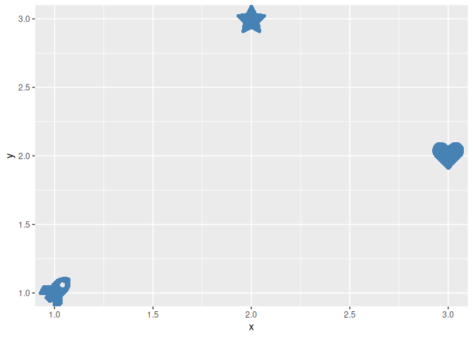

Mapping data to icons

If the icon aesthetic is already mapped to icon values, scale_icon_identity() passes them through unchanged. To map a discrete data column (e.g. a category) to an icon instead, use scale_icon_manual(). There’s no automatic discrete palette for icons, so values is always required. Since icon vectors can’t be named, values is matched positionally against the sorted data levels by default; pass limits to match against a different order instead:

df <- data.frame(
  x = 1:3, y = c(1, 3, 2),
  type = c("rocket", "star", "heart")
)
ggplot(df, aes(x, y, icon = type, colour = type)) +
  geom_icon(size = 12) +
  scale_icon_manual(
    limits = c("rocket", "star", "heart"),
    values = c(
      fontawesome$solid$rocket,
      fontawesome$solid$star,
      fontawesome$solid$heart
    )
  ) +
  scale_colour_manual(
    limits = c("rocket", "star", "heart"),
    values = c(rocket = "steelblue", star = "goldenrod", heart = "firebrick")
  )

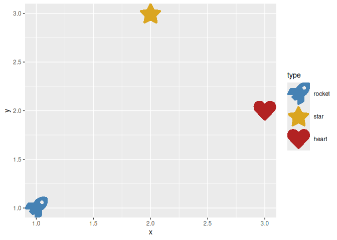
Icons drawn with geom_icon() also appear as their own legend key glyph, via draw_key_icon(), so the legend shows the actual icon shape instead of a generic point.

Annotating a plot with a fixed-position icon

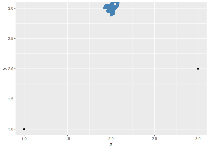
annotation_icon() adds one or more icons at fixed (x, y) positions, the icon analogue of annotate(). Unlike annotation_custom(), it does train the panel’s position scales, so placing an icon outside the data’s range still expands the axes to fit it:

ggplot(data.frame(x = 1:3, y = c(1, 3, 2)), aes(x, y)) +
  geom_point() +
  annotation_icon(
    icon = fontawesome$solid$rocket,
    x = 2, y = 3, size = 14, colour = "steelblue"
  )

Icons as axis, strip and legend labels

element_icon() is a theme() element, parallel to element_text(), for use in axis.text, strip.text, legend.text and similar text-drawing theme settings. Any label matching a name in its icons lookup is drawn as that icon; every other label falls back to ordinary text:

battery <- list(
  `4` = fontawesome$solid$`battery-quarter`,
  `6` = fontawesome$solid$`battery-half`,
  `8` = fontawesome$solid$`battery-full`
)

ggplot(mtcars, aes(factor(cyl), mpg)) +
  geom_boxplot() +
  labs(x = "Cylinders") +
  theme(axis.text.x = element_icon(icons = battery, size = 16))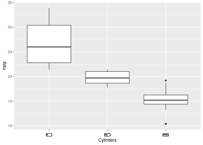

Isotype charts with geom_pictogram()

geom_pictogram() draws a value as a grid of repeated icons, some fraction of them filled in and the rest left faded, the way an isotype chart uses “each icon = n units” instead of a bar’s length. Leaving y out of aes() grows the grid upward like a column chart, with value mapped to how many icons are filled and icon/colour mapped to category:

commutes <- data.frame(mode = c("Bicycle", "Car"), count = c(890, 1230))
ggplot(commutes, aes(mode, value = count, icon = mode, colour = mode)) +
  geom_pictogram(ncol = 5) +
  scale_icon_manual(values = c(fontawesome$solid$bicycle, fontawesome$solid$car)) +
  scale_colour_manual(values = c("steelblue", "firebrick")) +
  labs(x = NULL, value = "commuters")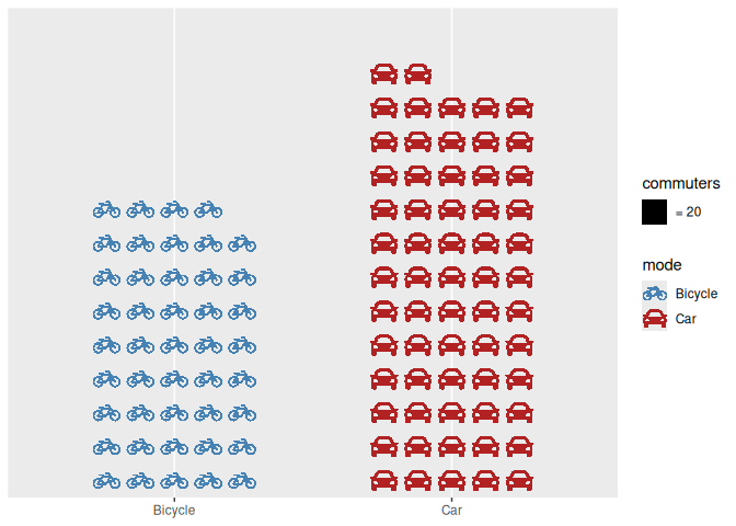

Each icon stands for a fixed amount (here, 20 commuters); guide_pictogram() spells this ratio out in the legend automatically.

These binaries (installable software) and packages are in development.
They may not be fully stable and should be used with caution. We make no claims about them.