
The hardware and bandwidth for this mirror is donated by METANET, the Webhosting and Full Service-Cloud Provider.
If you wish to report a bug, or if you are interested in having us mirror your free-software or open-source project, please feel free to contact us at mirror[@]metanet.ch.
The Tissot Indicatrix characterizes local distortion in map projections. This package computes and plots indicatrixes using the PROJ library directly via the PROJ R package.
Derived (with permission) from Bill Huber’s GIS StackExchange answer.
# install.packages("pak")
pak::pak("tissot")tissot() returns a tibble of distortion properties. The
second argument is the projection target;
source defaults to EPSG:4326:
library(tissot)
tissot(c(147, -42), "+proj=utm +zone=55 +south")
#> Tissot indicatrix: 1 point, +proj=utm +zone=55 +south
#> # A tibble: 1 × 14
#>       x     y dx_dlam dy_dlam    dx_dphi dy_dphi
#>   <dbl> <dbl>   <dbl>   <dbl>      <dbl>   <dbl>
#> 1   147   -42 0.74396       0 6.1410e-16 0.99739
#> # ℹ 8 more variables: scale_h <dbl>, scale_k <dbl>,
#> #   scale_omega <dbl>, scale_a <dbl>, scale_b <dbl>,
#> #   scale_area <dbl>, angle_deformation <dbl>,
#> #   convergence <dbl>
Columns include: scale_h (meridional),
scale_k (parallel), scale_a /
scale_b (max/min singular values), scale_area,
angle_deformation, and convergence.
indicatrix() builds plottable ellipses. The dashed
circle is the undistorted reference; the filled ellipse shows the
projection’s distortion.
xy <- expand.grid(x = seq(0, 1e6, length.out = 5), y = seq(4900000, 5700000, length.out = 4))
lonlat <- tissot_unproject(xy, source = "+proj=utm +zone=55 +south")
tis <- tissot(lonlat, "+proj=utm +zone=55 +south")
plot(indicatrix(tis), scale = 3e4)
tissot_map()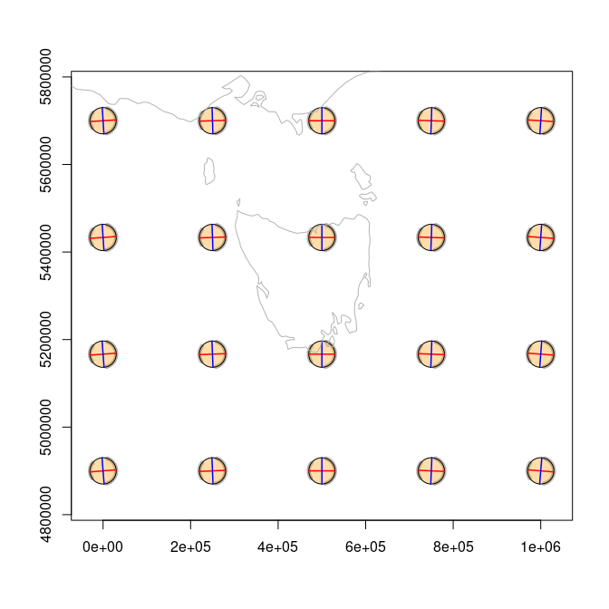
plot of chunk utm55
What does that top left indicatrix look like?
plot(indicatrix(tis)[1])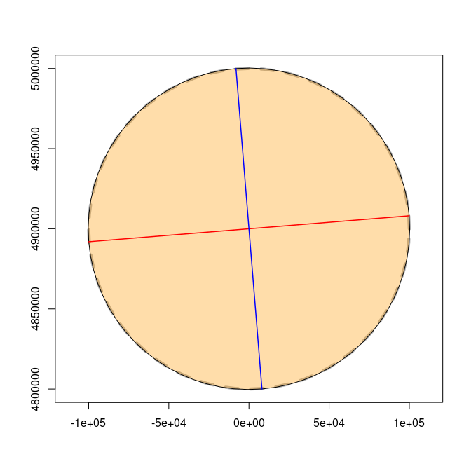
plot of chunk topleft
Far from our UTM zone we are in a lot more trouble.
## UTM zone 55 is at 147 longitude (55 * 6 - 183)
tis <- tissot(cbind(100, -42), "+proj=utm +zone=55 +south")
plot(indicatrix(tis))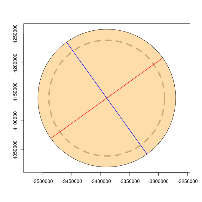
plot of chunk very-bad-trouble
##  In Mercator we have well known problems
tis <- tissot(cbind(147, -42), "+proj=merc")
plot(indicatrix(tis))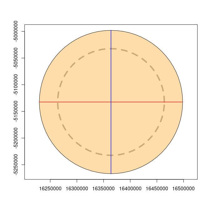
plot of chunk very-bad-trouble
## close to the equator Mercator is ok (in exactly the same way that UTM Zone 55 is ok near 147E longitude)
tis <- tissot(cbind(147, 0), "+proj=merc")
plot(indicatrix(tis))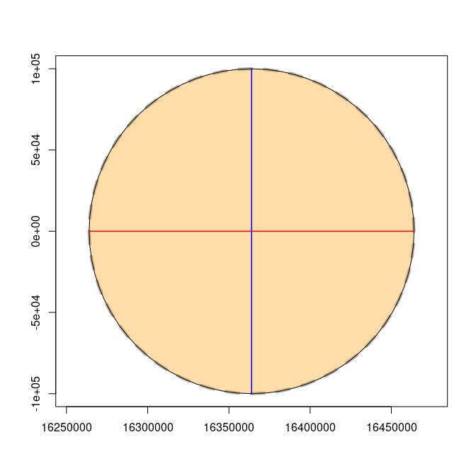
plot of chunk very-bad-trouble
Map projection is arbitrary.
xy <- expand.grid(seq(-150, 150, by = 30), seq(-60, 60, by = 30))
r <- tissot(xy, "+proj=robin")
ii <- indicatrix(r)
plot(ii, scale = 6e5, add = FALSE, show.axes  = TRUE, show.circle = TRUE)
tissot_map()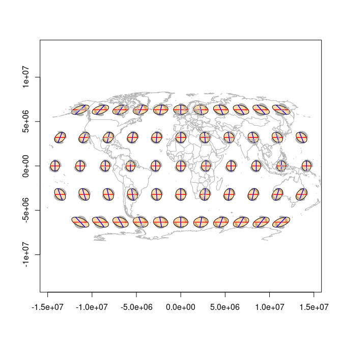
plot of chunk robinson
summary(r)
#> Tissot indicatrix: 55 points
#>   Source CRS: EPSG:4326
#>   Target CRS: +proj=robin
#>   Areal scale:  min=0.8154  max=1.2004  mean=1.0095
#>   Angular def:  min=1.9369  max=51.8469  mean=21.3801 deg
#>   Scale h:      min=0.8856  max=1.3030  (meridional)
#> Scale k: min=0.8487 max=1.3555 (parallel)Pass fill.by to colour ellipses by a distortion
metric:
plot(ii, scale = 6e5, add = FALSE, fill.by = "scale_area")
tissot_map()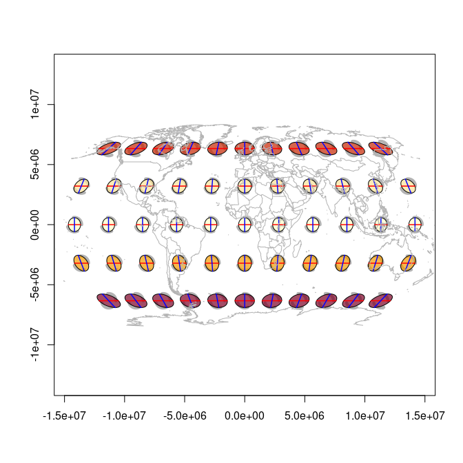
plot of chunk coloured
plot(ii, scale = 6e5, add = FALSE, fill.by = "angle_deformation")
tissot_map()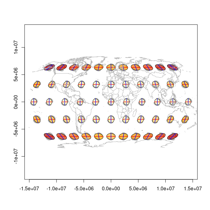
plot of chunk angle_deformation
m <- tissot(xy, "+proj=moll")
plot(indicatrix(m), scale = 5e5, add = FALSE)
tissot_map()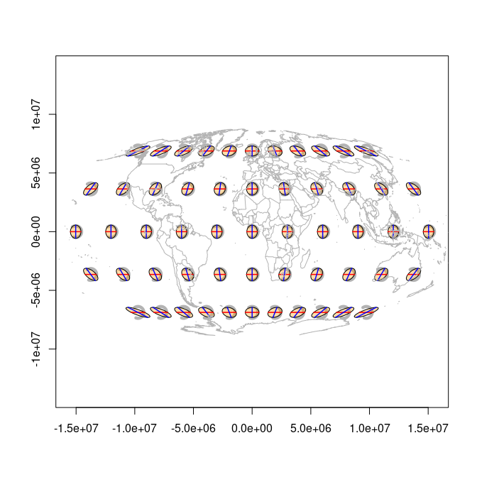
plot of chunk mollweide
merc_xy <- expand.grid(seq(-150, 150, by = 30), seq(-75, 75, by = 15))
me <- tissot(merc_xy, "+proj=merc")
plot(indicatrix(me), scale = 5e5, add = FALSE)
tissot_map()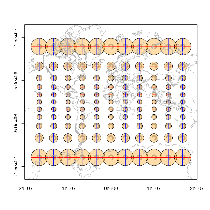
plot of chunk mercator
A single indicatrix with axes and reference circle:
ii2 <- indicatrix(c(147, -42), "+proj=lcc +lat_1=-36 +lat_2=-38 +lat_0=-37 +lon_0=145")
plot(ii2[[1]], scale = 1e4, add = FALSE, show.axes = TRUE, show.circle = TRUE)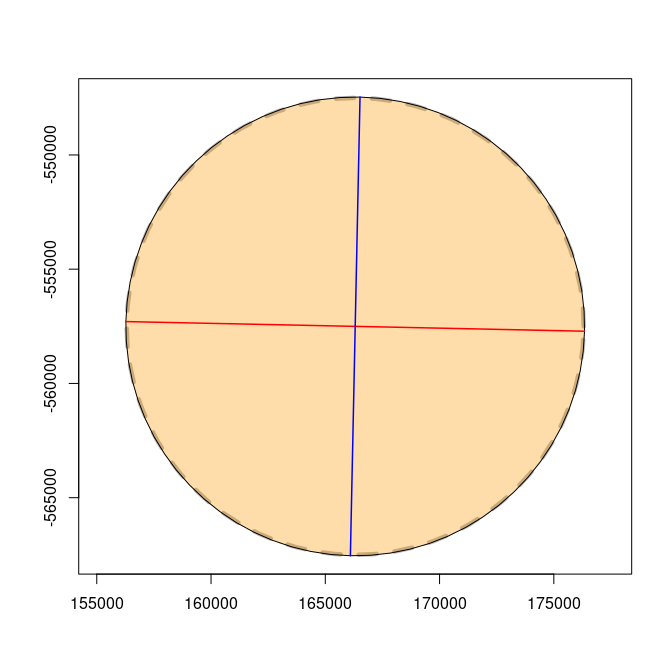
plot of chunk single2
ii3 <- indicatrix(c(147, -42), "+proj=lcc +lat_1=-15 +lat_2=5 +lat_0=0 +lon_0=145")
plot(ii3[[1]], scale = 1e4, add = FALSE, show.axes = TRUE, show.circle = TRUE)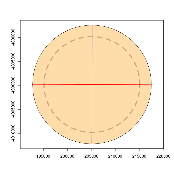
plot of chunk single3
Lambert Conformal Conic
pxy <- expand.grid(seq(100, 200, by = 25), seq(-75, -45, by = 10))
p <- tissot(pxy, "+proj=lcc +lat_0=-60 +lon_0=147 +lat_1=-70 +lat_2=-55")
plot(indicatrix(p), scale = 3e5, add = FALSE, fill.by = "scale_area")
tissot_map()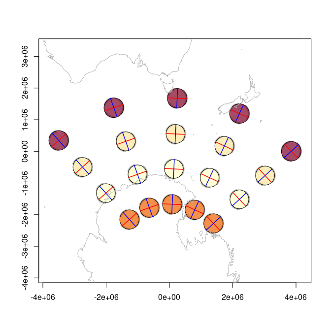
plot of chunk lcc
Universal Transverse Mercator
qxy <- expand.grid(seq(100, 200, by = 25), seq(-75, -45, by = 10))
p <- tissot(qxy, "EPSG:32755")
plot(indicatrix(p), scale = 3e5, add = FALSE, fill.by = "scale_area")
tissot_map()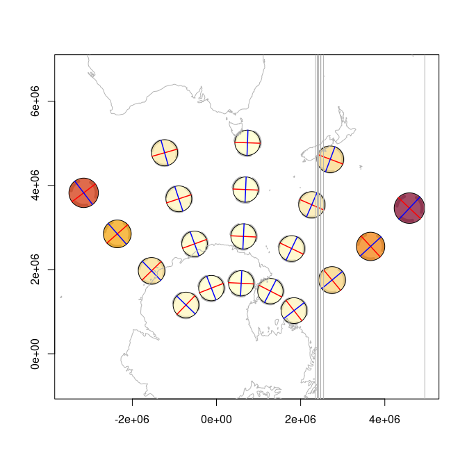
plot of chunk utm
In any projection we should refer to a regular grid of points in its crs, else we get weird situations like this, more obvious on an actual pole:
polar_xy <- expand.grid(seq(-180, 150, by = 30), seq(-80, -50, by = 10))
p <- tissot(polar_xy, "+proj=stere +lat_0=-90 +lon_0=147")
plot(indicatrix(p), scale = 2.5e5, add = FALSE, fill.by = "scale_area")
tissot_map()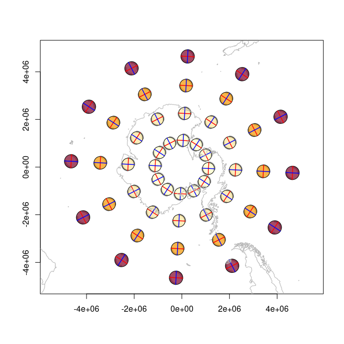
plot of chunk polar
la <- tissot(polar_xy, "+proj=laea +lat_0=-90 +lon_0=147")
plot(indicatrix(la), scale = 2.5e5, add = FALSE)
tissot_map()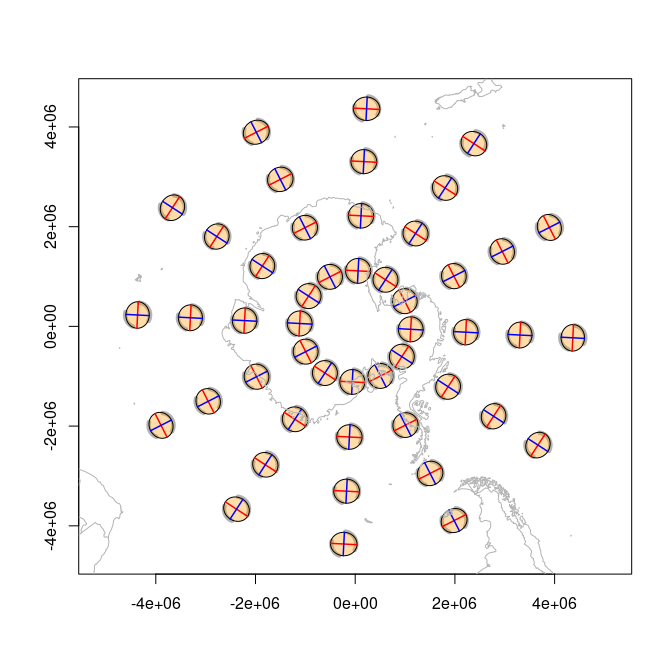
plot of chunk laea
If we push the centre away from the pole in Azimuthal Equidistant, it’s useful to see what happens.
lea <- tissot(polar_xy, "+proj=aeqd +lat_0=-20 +lon_0=147")
plot(indicatrix(lea), scale = 2.5e5, add = FALSE)
tissot_map()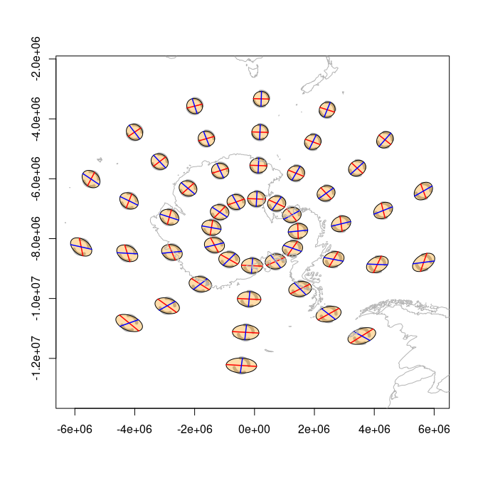
plot of chunk aeqd
As with the UTM example above, using tissot_unproject()
it is usually far better to generate a grid in the CRS being assessed. A
grid in lon/lat won’t be very meaningful in many projections.
op <- par(mfrow = c(1, 2))
ext <- c(-180, 150, -80, -50)
crs <- "+proj=stere +lat_0=-90 +lon_0=147"

projext <- reproj::reproj_extent(ext, crs, source = "EPSG:4326")
polar <- expand.grid(seq(projext[1L], projext[2L], by = 30 * 1e5), seq(projext[3L], projext[4L], by = 10 * 1e5))
polar_xy <- tissot_unproject(polar, "EPSG:4326", source = crs)
p <- tissot(polar_xy, crs, source = "EPSG:4326")
plot(indicatrix(p), scale = 2.5e5, add = FALSE, fill.by = "scale_area")
tissot_map()

ext <- c(-180, 150, -80, -50)
crs <- "+proj=laea +lat_0=-90 +lon_0=147"
projext <- reproj::reproj_extent(ext, crs, source = "EPSG:4326")

polar <- expand.grid(seq(projext[1L], projext[2L], by = 30 * 1e5), seq(projext[3L], projext[4L], by = 10 * 1e5))
polar_xy <- tissot_unproject(polar, "EPSG:4326", source = crs)
p <- tissot(polar_xy, crs, source = "EPSG:4326")
plot(indicatrix(p), scale = 2.5e5, add = FALSE, fill.by = "scale_area")
tissot_map()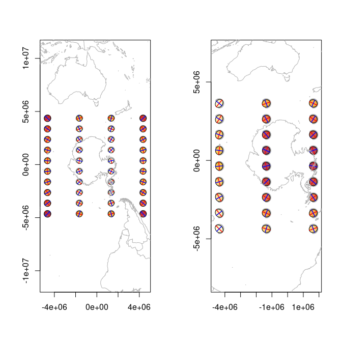
plot of chunk polar-proj
par(op)Most “Tissot indicatrix” plots you’ll find online are just geographic circles drawn on the map. They show what happens to a circle under the projection, which is useful — but it’s not the indicatrix. The indicatrix is the Jacobian of the projection at a point: it gives you actual scale factors, angular deformation, and areal distortion. This package computes those.
Other examples: mgimond.
Please note that the tissot project is released with a Contributor Code of Conduct. By contributing to this project, you agree to abide by its terms.
These binaries (installable software) and packages are in development.
They may not be fully stable and should be used with caution. We make no claims about them.