
The hardware and bandwidth for this mirror is donated by METANET, the Webhosting and Full Service-Cloud Provider.
If you wish to report a bug, or if you are interested in having us mirror your free-software or open-source project, please feel free to contact us at mirror[@]metanet.ch.
Performs the Baumgartner-Weiß-Schindler 2-sample test of equal probability distributions.
– Steven E. Pav, shabbychef@gmail.com
This package can be installed from CRAN, via drat, or from github:
# via CRAN:
install.packages("BWStest")
# via drat:
if (require(drat)) {
    drat:::add("shabbychef")
    install.packages("BWStest")
}
# get snapshot from github (may be buggy)
if (require(devtools)) {
    install_github("shabbychef/BWStest")
}The Baumgartner-Weiß-Schindler (‘BWS’) test is a non-parametric hypothesis test for the null of equal probability distributions of two samples, not unlike the two-sample Kolmogorov-Smirnov test or the Wilcoxon test. The BWS test is more powerful than these other tests under certain alternatives, as shown in the original paper and replicated below.
The front end for the hypothesis test is the function
bws_test. By default it supports the the classical
Baumgartner-Weiß-Schindler test for a two-sided alternative, returning a
htest object:
require(BWStest)
set.seed(12345)
# under the null:
x <- rnorm(200)
y <- rnorm(200)
hval <- bws_test(x, y)
show(hval)
##
## two-sample BWS test
##
## data: x vs. y
## B = 1, p-value = 0.2
## alternative hypothesis: true difference in survival functions is not equal to 0# under the alternative:
z <- rnorm(200, mean = 1)
hval <- bws_test(x, z)
show(hval)##
## two-sample BWS test
##
## data: x vs. z
## B = 30, p-value <2e-16
## alternative hypothesis: true difference in survival functions is not equal to 0The code also supports alternative test statistics from Neuhäuser and Murakami, along with supporting one-sided alternatives for some of the tests:
set.seed(12345)
# under the alternative:
x <- rnorm(200)
y <- rnorm(200, mean = 1)
hval <- bws_test(x, z, alternative = "less")
show(hval)
##
## two-sample Neuhauser/Murakami test
##
## data: x vs. z
## B_2 = -30, p-value <2e-16
## alternative hypothesis: true difference in survival functions is less than 0x <- rnorm(8)
y <- rnorm(8, mean = 1)
hval <- bws_test(x, z, method = "B3", alternative = "two.sided")
show(hval)##
## two-sample Murakami test
##
## data: x vs. z
## B_3 = 2, p-value = 0.009
## alternative hypothesis: true difference in survival functions is not equal to 0We should note that the B3 through B5 tests
do not achieve nominal coverage for large sample sizes and
should only be used on sample sizes of about 12 or fewer in
each of the two samples.
Doverai No Proverai (Trust, but verify.) – Russian proverb.
Here we perform 5000 simulations of the BWS test under the null hypothesis, then compute the CDF of the test statistic. If the code is correct, the resultant p-values should be uniform. So I q-q plot under the uniform law:
require(BWStest)

# now compute a bunch under the null:
set.seed(1234)
bvals <- replicate(5000, bws_stat(rnorm(100), rnorm(100)))
# compute the approximate p-values under the null:
pvals <- bws_cdf(bvals)

require(ggplot2)
ph <- ggplot(data.frame(pv = pvals), aes(sample = pv)) +
    stat_qq(distribution = stats::qunif)
print(ph)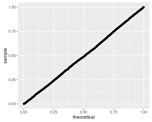
Looks good to me!
Here we replicate figure 2A of Baumgartner et al. We draw two samples from the normal distribution, both with unit standard deviation, letting a be the difference in means. We check the empirical rejection rate at the 0.05 level for a few different tests. As in Baumgartner, we find that the lowly t-test is the most powerful in this case, with the BWS, Cramer-Von Mises, and Wilcoxon tests displaying similar power, then the KS test the least powerful. Note that the Kolmogorov Smirnov test does not appear to have nominal coverage under the null, probably due to the small sample size.
n.sim <- 10000
avals <- seq(0, 3.2, length.out = 17)
alpha <- 0.05
mnsize <- 10

# this is archived on CRAN, unfortunately:
library(CvM2SL2Test)
# find the CVM critical value.
critv <- uniroot(function(x) {
    cvmts.pval(x, mnsize, mnsize) - alpha
}, lower = 0, upper = 100, maxiter = 5000)$root

set.seed(1234)
simul <- sapply(avals, function(a) {
    rejs <- replicate(n.sim, {
        x <- rnorm(mnsize, mean = 0)
        y <- rnorm(mnsize, mean = a)
        bws <- bws_cdf(bws_stat(x, y), lower_tail = FALSE) <=
            alpha
        ttv <- t.test(x, y, alternative = "two.sided")$p.value <=
            alpha
        cvm <- cvmts.test(x, y) >= critv
        ksv <- ks.test(x, y, alternative = "two.sided")$p.value <=
            alpha
        wcx <- wilcox.test(x, y, alternative = "two.sided")$p.value <=
            alpha
        c(bws, ttv, cvm, ksv, wcx)
    })
    rejrate <- rowMeans(rejs)
    names(rejrate) <- c("BWS test", "t test", "Cramer-Von Mises test",
        "Kolmogorov Smirnov test", "Wilcoxon test")
    rejrate
}, simplify = "matrix")

Arejrates <- data.frame(t(simul))
Arejrates$a <- avalslibrary(tidyr)
library(dplyr)
library(ggplot2)
plotdf <- tidyr::gather(Arejrates, "test", "rejection_rate",
-a) %>% dplyr::mutate(test = gsub("\\.", " ", test))
ph <- ggplot(plotdf, aes(x = a, y = rejection_rate,
group = test, colour = test)) + geom_line() + geom_point() +
labs(x = "a, difference in means", y = "rejection rate")
print(ph)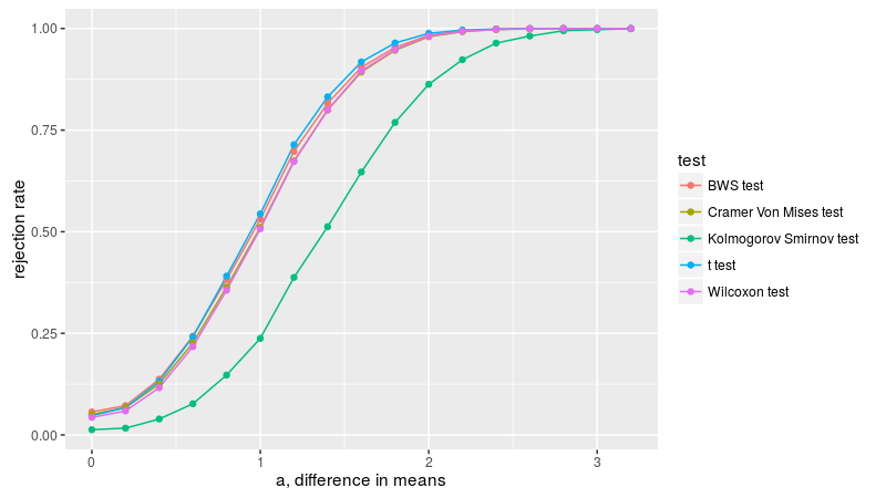
Here we replicate figure 2B of Baumgartner et al. We draw two samples from the normal distribution, both with zero mean, one with unit standard deviation, the other with standard deviation of sigma. We compute the empirical rejection rate at the 0.05 level, dropping the t-test since it is not relevant for this formulation. As in Baumgartner, we find the BWS test is the most powerful, followed by KS test, then Cramer-Von Mises, then Wilcoxon, which is basically useless in this simulation.
n.sim <- 10000
svals <- seq(1, 45, length.out = 10)
alpha <- 0.05
mnsize <- 10

# this is archived on CRAN, unfortunately:
library(CvM2SL2Test)
# find the CVM critical value.
critv <- uniroot(function(x) {
    cvmts.pval(x, mnsize, mnsize) - alpha
}, lower = 0, upper = 100, maxiter = 5000)$root

set.seed(1234)
simul <- sapply(svals, function(s) {
    rejs <- replicate(n.sim, {
        x <- rnorm(mnsize, mean = 0, sd = 1)
        y <- rnorm(mnsize, mean = 0, sd = s)
        bws <- bws_cdf(bws_stat(x, y), lower_tail = FALSE) <=
            alpha
        cvm <- cvmts.test(x, y) >= critv
        ksv <- ks.test(x, y, alternative = "two.sided")$p.value <=
            alpha
        wcx <- wilcox.test(x, y, alternative = "two.sided")$p.value <=
            alpha
        c(bws, cvm, ksv, wcx)
    })
    rejrate <- rowMeans(rejs)
    names(rejrate) <- c("BWS test", "Cramer-Von Mises test",
        "Kolmogorov Smirnov test", "Wilcoxon test")
    rejrate
}, simplify = "matrix")

Brejrates <- data.frame(t(simul))
Brejrates$sigma <- svals
plotdf <- tidyr::gather(Brejrates, "test", "rejection_rate",
-sigma) %>% dplyr::mutate(test = gsub("\\.", " ",
test))
ph <- ggplot(plotdf, aes(x = sigma, y = rejection_rate,
group = test, colour = test)) + geom_line() + geom_point() +
labs(x = "sigma, ratio of standard deviations",
y = "rejection rate")
print(ph)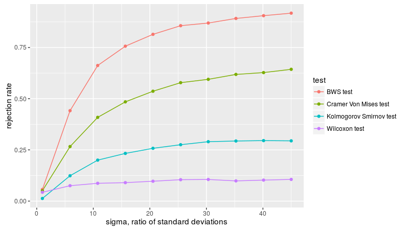
Here we replicate figure 3A of Baumgartner et al. We draw two samples from the exponential distribution, letting l be the ratio of the rate parameters of the two populations. We compute the empirical rejection rate at the 0.05 level. As in Baumgartner, we find the BWS test is the most powerful, followed by Wilcoxon, then Cramer-Von Mises, then the KS test.
n.sim <- 10000
lvals <- seq(1, 12)
alpha <- 0.05
mnsize <- 10

# this is archived on CRAN, unfortunately:
library(CvM2SL2Test)
# find the CVM critical value.
critv <- uniroot(function(x) {
    cvmts.pval(x, mnsize, mnsize) - alpha
}, lower = 0, upper = 100, maxiter = 5000)$root

set.seed(1234)
simul <- sapply(lvals, function(l) {
    rejs <- replicate(n.sim, {
        x <- rexp(mnsize, rate = 1)
        y <- rexp(mnsize, rate = l)
        bws <- bws_cdf(bws_stat(x, y), lower_tail = FALSE) <=
            alpha
        cvm <- cvmts.test(x, y) >= critv
        ksv <- ks.test(x, y, alternative = "two.sided")$p.value <=
            alpha
        wcx <- wilcox.test(x, y, alternative = "two.sided")$p.value <=
            alpha
        c(bws, cvm, ksv, wcx)
    })
    rejrate <- rowMeans(rejs)
    names(rejrate) <- c("BWS test", "Cramer-Von Mises test",
        "Kolmogorov Smirnov test", "Wilcoxon test")
    rejrate
}, simplify = "matrix")

Crejrates <- data.frame(t(simul))
Crejrates$lratio <- lvals
plotdf <- tidyr::gather(Crejrates, "test", "rejection_rate",
-lratio) %>% dplyr::mutate(test = gsub("\\.", " ",
test))
ph <- ggplot(plotdf, aes(x = lratio, y = rejection_rate,
group = test, colour = test)) + geom_line() + geom_point() +
labs(x = "l, ratio of rate parameters", y = "rejection rate")
print(ph)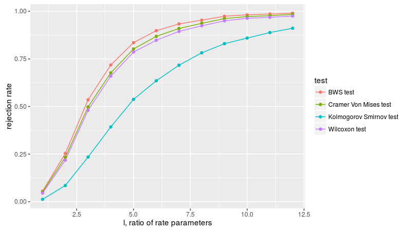
Here we replicate figure 3B of Baumgartner et al. We draw two samples, one from the normal distribution with zero mean and variance one-twelth, the other uniformly on -0.5 to 0.5. We take equal sample sizes from these two populations, then vary the sample size, checking the empirical rejection rate at the 0.05 level. Since the first two moments are equal, the Wilcoxon test is useless here, and not applied. As in Baumgartner, we find the BWS test is the most powerful, followed by the KS test and Cramer-Von Mises tests. Based on the power plots here, I theorize that Baumgartner et al. are plotting the total sample sizes on the x axis, that is, drawing n from both distributions, then plotting empirical power versus 2n. We follow that convention, which makes the plots match those of Baumgartner.
n.sim <- 10000
mvals <- seq(10, 670, by = 60)
alpha <- 0.05

# this is archived on CRAN, unfortunately:
library(CvM2SL2Test)

set.seed(1234)
simul <- sapply(mvals, function(mnsize) {
    # find the CVM critical value.  note that this
    # basically converged for mnsize > 100 or so, so we
    # take the min..  for reasons of speed.
    critv <- uniroot(function(x) {
        cvmts.pval(x, min(mnsize, 80), min(mnsize,
            80)) - alpha
    }, lower = 0, upper = 2, maxiter = 100)$root
    rejs <- replicate(n.sim, {
        x <- rnorm(mnsize, mean = 0, sd = 1/sqrt(12))
        y <- runif(mnsize, min = -0.5, max = 0.5)
        bws <- bws_cdf(bws_stat(x, y), lower_tail = FALSE) <=
            alpha
        cvm <- cvmts.test(x, y) >= critv
        ksv <- ks.test(x, y, alternative = "two.sided")$p.value <=
            alpha
        c(bws, cvm, ksv)
    })
    rejrate <- rowMeans(rejs)
    names(rejrate) <- c("BWS test", "Cramer-Von Mises test",
        "Kolmogorov Smirnov test")
    rejrate
}, simplify = "matrix")

Drejrates <- data.frame(t(simul))
Drejrates$ssize <- 2 * mvals
plotdf <- tidyr::gather(Drejrates, "test", "rejection_rate",
-ssize) %>% dplyr::mutate(test = gsub("\\.", " ",
test))
ph <- ggplot(plotdf, aes(x = ssize, y = rejection_rate,
group = test, colour = test)) + geom_line() + geom_point() +
labs(x = "m+n, total sample size", y = "rejection rate")
print(ph)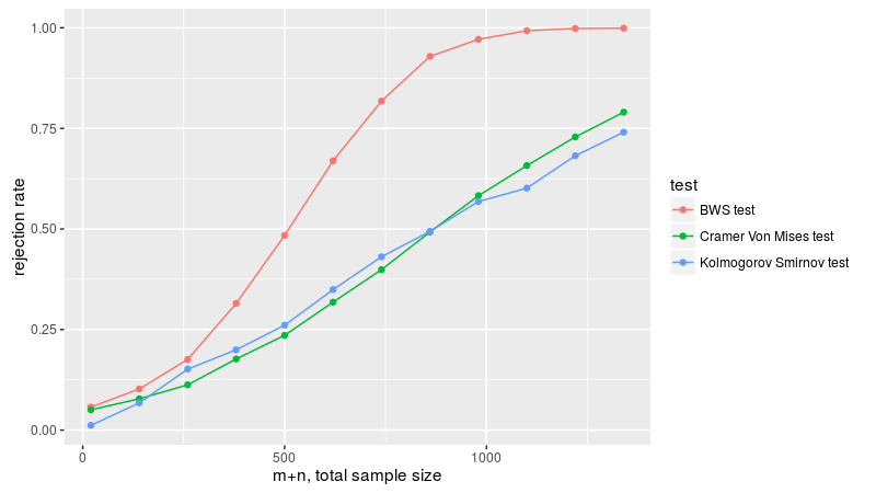
Neuhäuser and Murakami
described some modifications to the original test of Baumgartner.
Neuhäuser’s test allows one to test against directional alternatives.
Murakami enumerated some modifications to the weighting scheme. These
are available via the murakami_stat function, where the
flavor corresponds to the test number from Murakami’s
paper, namely
Here we take these through the paces as above.
As above, we draw samples under the null and compare to the putative CDF function
require(BWStest)

# now compute a bunch under the null:
n1 <- 9
n2 <- n1
set.seed(1234)
allpvs <- lapply(0L:5L, function(flavor) {
    bvals <- replicate(5000, murakami_stat(rnorm(n1),
        rnorm(n2), flavor = flavor))
    # compute the approximate p-values under the null:
    pvals <- murakami_cdf(bvals, n1 = n1, n2 = n2,
        flavor = flavor)
    data.frame(pv = pvals, flavor = flavor)
})

df <- do.call(rbind, allpvs)

require(ggplot2)
ph <- ggplot(df, aes(sample = pv)) + facet_grid(flavor ~
    .) + stat_qq(distribution = stats::qunif)
print(ph)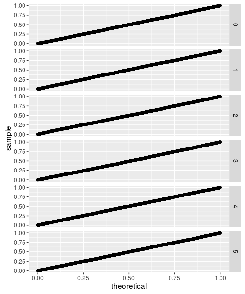
While these all look fine, they are based on small sample sizes. The CDF is approximated by evaluating all the permutations (with memoisation to tame the computational requirements), but this can only be done up to some reasonably small sample size. If the test statistic does not converge beyond that sample size, the CDF approximation will not be accurate. This appears to be the case for flavors 3 through 5, as demonstrated below:
require(BWStest)

# now compute a bunch under the null:
n1 <- 50
n2 <- n1
set.seed(1234)
allpvs <- lapply(0L:5L, function(flavor) {
    bvals <- replicate(5000, murakami_stat(rnorm(n1),
        rnorm(n2), flavor = flavor))
    # compute the approximate p-values under the null:
    pvals <- murakami_cdf(bvals, n1 = n1, n2 = n2,
        flavor = flavor)
    data.frame(pv = pvals, flavor = flavor)
})

df <- do.call(rbind, allpvs)

require(ggplot2)
ph <- ggplot(df, aes(sample = pv)) + facet_grid(flavor ~
    .) + stat_qq(distribution = stats::qunif)
print(ph)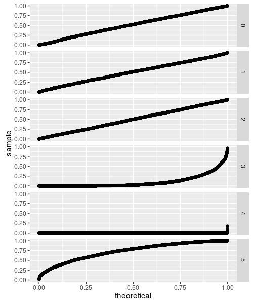
So that’s not so great.
We can perform the power comparisons of Baumgartner et al. using the Murakami test statistics. Here we consider the setup of figure 2A, samples of size 10 from the normal distribution with equal variances but different means. Neuhäuser’s test is, as expected, more powerful for detecting this one-sided alternative, probably on par with the t-test, while the BWS test (basically equivalent to Murakami 1) is next, then 5, 3, 4.
n.sim <- 10000
avals <- seq(0, 3.2, length.out = 17)
alpha <- 0.05
mnsize <- 10

set.seed(1234)
simul <- sapply(avals, function(a) {
    statvs <- replicate(n.sim, {
        x <- rnorm(mnsize, mean = 0)
        y <- rnorm(mnsize, mean = a)
        bws <- bws_stat(x, y)
        murav <- sapply(1L:5L, function(flavor) {
            murakami_stat(x, y, flavor = flavor)
        })
        c(bws, murav)
    })
    rej_bws <- mean(bws_cdf(statvs[1, ], lower_tail = FALSE) <=
        alpha)
    rej_mur <- sapply(2:6, function(rown) {
        mean(murakami_cdf(statvs[rown, ], mnsize, mnsize,
            flavor = rown - 1, lower_tail = FALSE) <=
            alpha)
    })

    rejrate <- c(rej_bws, rej_mur)
    names(rejrate) <- c("BWS test", "Murakami 1", "Neuhauser",
        "Murakami 3", "Murakami 4", "Murakami 5")
    rejrate
}, simplify = "matrix")

Arejrates <- data.frame(t(simul))
Arejrates$a <- avalslibrary(tidyr)
library(dplyr)
library(ggplot2)
plotdf <- tidyr::gather(Arejrates, "test", "rejection_rate",
-a) %>% dplyr::mutate(test = gsub("\\.", " ", test))
ph <- ggplot(plotdf, aes(x = a, y = rejection_rate,
group = test, colour = test)) + geom_line() + geom_point() +
labs(x = "a, difference in means", y = "rejection rate")
print(ph)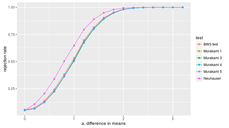
Now we consider figure2B, with two samples of equal size from the normal distribution with zero mean, but different standard deviations. Neuhäuser’s test is nearly useless here because the means of the populations are equal. Murakami 3, 4, and 5 are the most powerful, followed by BWS.
n.sim <- 10000
svals <- seq(1, 45, length.out = 10)
alpha <- 0.05
mnsize <- 10

set.seed(1234)
simul <- sapply(svals, function(s) {
    statvs <- replicate(n.sim, {
        x <- rnorm(mnsize, mean = 0, sd = 1)
        y <- rnorm(mnsize, mean = 0, sd = s)
        bws <- bws_stat(x, y)
        murav <- sapply(1L:5L, function(flavor) {
            murakami_stat(x, y, flavor = flavor)
        })
        c(bws, murav)
    })
    rej_bws <- mean(bws_cdf(statvs[1, ], lower_tail = FALSE) <=
        alpha)
    rej_mur <- sapply(2:6, function(rown) {
        mean(murakami_cdf(statvs[rown, ], mnsize, mnsize,
            flavor = rown - 1, lower_tail = FALSE) <=
            alpha)
    })

    rejrate <- c(rej_bws, rej_mur)
    names(rejrate) <- c("BWS test", "Murakami 1", "Neuhauser",
        "Murakami 3", "Murakami 4", "Murakami 5")
    rejrate
}, simplify = "matrix")

Brejrates <- data.frame(t(simul))
Brejrates$sigma <- svals
plotdf <- tidyr::gather(Brejrates, "test", "rejection_rate",
-sigma) %>% dplyr::mutate(test = gsub("\\.", " ",
test))
ph <- ggplot(plotdf, aes(x = sigma, y = rejection_rate,
group = test, colour = test)) + geom_line() + geom_point() +
labs(x = "sigma, ratio of standard deviations",
y = "rejection rate")
print(ph)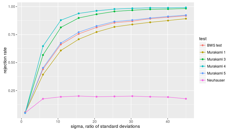
Now to figure 3A, with two equal sized samples from the exponential distribution, letting l be the ratio of the rate parameters of the two populations. The BWS test is the most powerful here, apparently.
n.sim <- 10000
lvals <- seq(1, 12)
alpha <- 0.05
mnsize <- 10

set.seed(1234)
simul <- sapply(lvals, function(l) {
    statvs <- replicate(n.sim, {
        x <- rexp(mnsize, rate = 1)
        y <- rexp(mnsize, rate = l)
        bws <- bws_stat(x, y)
        murav <- sapply(1L:5L, function(flavor) {
            murakami_stat(x, y, flavor = flavor)
        })
        c(bws, murav)
    })
    rej_bws <- mean(bws_cdf(statvs[1, ], lower_tail = FALSE) <=
        alpha)
    rej_mur <- sapply(2:6, function(rown) {
        mean(murakami_cdf(statvs[rown, ], mnsize, mnsize,
            flavor = rown - 1, lower_tail = FALSE) <=
            alpha)
    })

    rejrate <- c(rej_bws, rej_mur)
    names(rejrate) <- c("BWS test", "Murakami 1", "Neuhauser",
        "Murakami 3", "Murakami 4", "Murakami 5")
    rejrate
}, simplify = "matrix")

Crejrates <- data.frame(t(simul))
Crejrates$lratio <- lvals
plotdf <- tidyr::gather(Crejrates, "test", "rejection_rate",
-lratio) %>% dplyr::mutate(test = gsub("\\.", " ",
test))
ph <- ggplot(plotdf, aes(x = lratio, y = rejection_rate,
group = test, colour = test)) + geom_line() + geom_point() +
labs(x = "l, ratio of rate parameters", y = "rejection rate")
print(ph)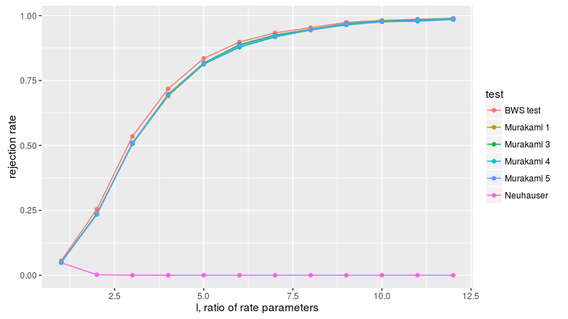
Now figure 3B, with a normal sample and a uniform sample, with equal first and second moments, varying the sample size. Because flavors 3 through 5 are not well behaved, we drop them here. Once again the BWS test is the most powerful.
n.sim <- 10000
mvals <- seq(10, 670, by = 60)
alpha <- 0.05

set.seed(1234)
simul <- sapply(mvals, function(mnsize) {
    statvs <- replicate(n.sim, {
        x <- rnorm(mnsize, mean = 0, sd = 1/sqrt(12))
        y <- runif(mnsize, min = -0.5, max = 0.5)
        bws <- bws_stat(x, y)
        murav <- sapply(1L:2L, function(flavor) {
            murakami_stat(x, y, flavor = flavor)
        })
        c(bws, murav)
    })
    rej_bws <- mean(bws_cdf(statvs[1, ], lower_tail = FALSE) <=
        alpha)
    rej_mur <- sapply(2:3, function(rown) {
        mean(murakami_cdf(statvs[rown, ], mnsize, mnsize,
            flavor = rown - 1, lower_tail = FALSE) <=
            alpha)
    })

    rejrate <- c(rej_bws, rej_mur)
    names(rejrate) <- c("BWS test", "Murakami 1", "Neuhauser")
    rejrate
}, simplify = "matrix")

Drejrates <- data.frame(t(simul))
Drejrates$ssize <- 2 * mvals
plotdf <- tidyr::gather(Drejrates, "test", "rejection_rate",
-ssize) %>% dplyr::mutate(test = gsub("\\.", " ",
test))
ph <- ggplot(plotdf, aes(x = ssize, y = rejection_rate,
group = test, colour = test)) + geom_line() + geom_point() +
labs(x = "m+n, total sample size", y = "rejection rate")
print(ph)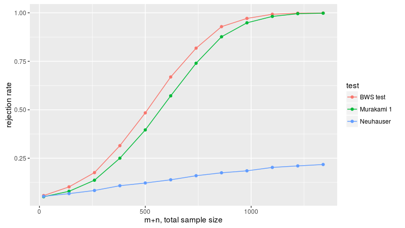
I anticipate the following:
These binaries (installable software) and packages are in development.
They may not be fully stable and should be used with caution. We make no claims about them.