The hardware and bandwidth for this mirror is donated by METANET, the Webhosting and Full Service-Cloud Provider.
If you wish to report a bug, or if you are interested in having us mirror your free-software or open-source project, please feel free to contact us at mirror[@]metanet.ch.
![]()
This platform is dedicated to the analysis of environmental mixture exposures and other mixture exposures with hierarchical gut microbiome outcome data. BaHZING, short for Bayesian Hierarchical Zero-Inflated Negative Binomial Regression with G-Computation, is a powerful toolkit designed to uncover intricate relationships between environmental exposures and gut microbiome outcomes.
You can install BaHZING from CRAN with:
# install.packages("BaHZING")Alternatively, you can install the development version of
BaHZING from GitHub:
# install.packages("pak")
pak::pak("Goodrich-Lab/BaHZING")The BaHZING formatting function requires a phyloseq object as the input. Ensure that your phyloseq object adheres to the required format. Refer to the phyloseq documentation for details on creating and manipulating phyloseq objects. For covariates in phyloseq object: All categorical covariates must be formatted as binary indicator variables rather than categorical or factor variables. For missing data: Ensure that there are no NA values in your data, perform the necessary filtering or imputation methods necessary to handle these values as BaHZING cannot function with missing data.
The formatting function produces an object that contains a table with all exposure variables, all covariates and the lowest level of microbiome outcome data. Additionally, the function produces binary matrices that represent the relationship between each level of microbiome data and the level above it.
The BaHZING model function provides results from the Bayesian hierarchical zero-inflated negative binomial regression model.
For a quick start, we utilize data from the iHMP publicly available data set. This example will guide you through the process of using BaHZING for analyzing environmental mixture exposures with hierarchical gut microbiome outcome data.
library(BaHZING)
#> Loading required package: rjags
#> Loading required package: coda
#> Linked to JAGS 4.3.2
#> Loaded modules: basemod,bugs
library(ggplot2)

### Load example data
data("iHMP_Reduced")

### Format microbiome data
formatted_data <- Format_BaHZING(iHMP_Reduced)

### Perform Bayesian hierarchical zero-inflated negative binomial regression with g-computation
### Specify a mixture of exposures
x <- c("soft_drinks_dietnum",
       "alcohol_dietnum",
       "fruit_juice_dietnum")
# "fruit_juice_dietnum","water_dietnum",
# "alcohol_dietnum","yogurt_dietnum","dairy_dietnum","probiotic_dietnum",
# "fruits_no_juice_dietnum", "vegetables_dietnum","beans_soy_dietnum",
# "whole_grains_dietnum","starch_dietnum", "eggs_dietnum",
# "processed_meat_dietnum","red_meat_dietnum","white_meat_dietnum",
# "shellfish_dietnum","fish_dietnum", "sweets_dietnum"

### Specify a set of covariates
covar <- c("consent_age")

### Perform BaH-ZING
# NOTE: For this example, we are using a small number of iterations to reduce
# the runtime. For a real analysis, we recommend using n.chain = 3,
# n.adapt, n.burnin, and n.sample > 5000.
bahzing_resout <- BaHZING_Model(formatted_data,
                         x = x,
                         covar = covar,
                         exposure_standardization = "none",
                         counterfactual_profiles = c(0,1),
                         n.chains = 1,
                         n.adapt = 60,
                         n.iter.burnin = 2,
                         n.iter.sample = 50)
#> #### Checking input data ####
#> Exposure and Covariate Data:
#> - Total sample size: 105
#> - Number of exposures: 3
#> Microbiome Data:
#> - Number of unique genus in data: 83
#> - Number of unique family in data: 13
#> - Number of unique order in data: 6
#> - Number of unique class in data: 5
#> - Number of unique phylum in data: 5
#> #### Running BaHZING with the following parameters ####
#> Exposure standardization: None
#> Compiling model graph
#>    Resolving undeclared variables
#>    Allocating nodes
#> Graph information:
#>    Observed stochastic nodes: 23310
#>    Unobserved stochastic nodes: 26980
#>    Total graph size: 350781
#>
#> Initializing model# Summarize the results
## Lets examine the Count model coefficients
count_estimates <- bahzing_resout[bahzing_resout$component == "Count model coefficients", ]
# Lets look at only the family level results
family_res_out <- count_estimates[count_estimates$domain == "Family",]
# Having a probabilty of direction > 0.975 is equivalent to examining
# whether the 95% BCI is overlapping with 0:
family_res_out$p_Dir_sig <- ifelse(family_res_out$pdir > 0.975,
"pDIR Sig", "pDIR Not Sig")
# Plot the genus results
ggplot(family_res_out, aes(x = estimate, y = taxa_name, color = p_Dir_sig)) +
geom_point() +
geom_errorbar(aes(xmin = bci_lcl, xmax = bci_ucl), width = 0) +
geom_vline(xintercept = 0, linetype = 2) +
facet_grid(~exposure) +
theme_classic() +
labs(title = "Family-level count model results",
x = "Log fold-change",
y = "Family",
color = "Probability of Direction")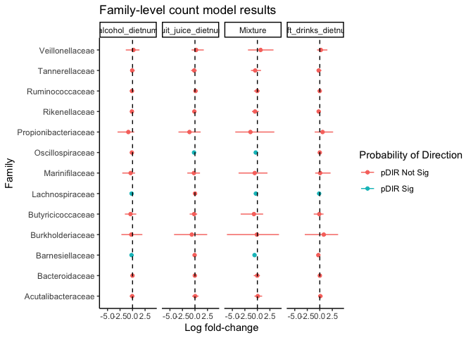
These binaries (installable software) and packages are in development.
They may not be fully stable and should be used with caution. We make no claims about them.