The hardware and bandwidth for this mirror is donated by METANET, the Webhosting and Full Service-Cloud Provider.
If you wish to report a bug, or if you are interested in having us mirror your free-software or open-source project, please feel free to contact us at mirror[@]metanet.ch.
| Resource | Github Actions | Code Coverage |
|---|---|---|
| Platforms | Windows, macOS, Linux | codecov |
| R CMD check |
Matching on generalized propensity scores with continuous exposures
CausalGPS is an R package that implements matching on
generalized propensity scores with continuous exposures. The package
introduces a novel approach for estimating causal effects using
observational data in settings with continuous exposures, and a new
framework for GPS caliper matching that jointly matches on both the
estimated GPS and exposure levels to fully adjust for confounding
bias.
library("devtools")
install_github("NSAPH-Software/CausalGPS")
library("CausalGPS")install.packages("CausalGPS")Developing Docker image can be downloaded from Docker Hub. See more details in docker_singularity.
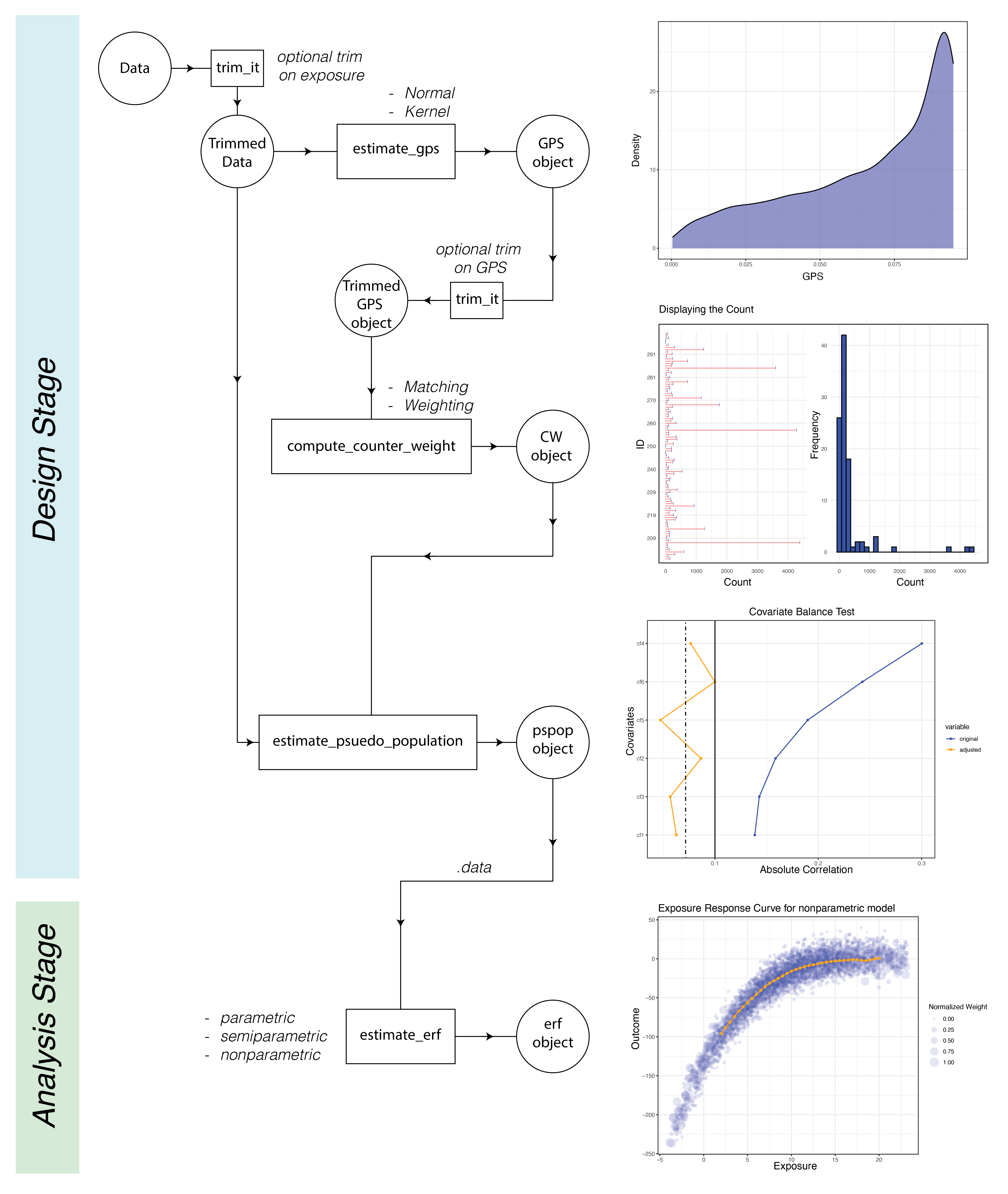
The CausalGPS package encompasses two primary stages: Design and Analysis. The Design stage comprises estimating GPS values, generating weights or counts of matched data, and evaluating the generated population. The Analysis stage is focused on estimating the exposure-response function. The following figure represents the process workflow

GPS values can be estimated using two distinct approaches:
kernel and normal.
set.seed(967)
m_d <- generate_syn_data(sample_size = 500)

m_xgboost <- function(nthread = 1,
                      ntrees = 35,
                      shrinkage = 0.3,
                      max_depth = 5,
                      ...) {SuperLearner::SL.xgboost(
                        nthread = nthread,
                        ntrees = ntrees,
                        shrinkage=shrinkage,
                        max_depth=max_depth,
                        ...)}

gps_obj <- estimate_gps(.data = m_d,
                        .formula = w ~ I(cf1^2) + cf2 + I(cf3^2) + cf4 + cf5 + cf6,
                        sl_lib = c("m_xgboost"),
                        gps_density = "normal")
where
.data A data.frame of input data including the
id column..formula The formula for modeling exposure based on
provided confounders.sl_lib A vector of prediction algorithms.gps_density A model type which is used for estimating
GPS value, including normal (default) and
kernel.The second step in processing involves computing the weight or count of matched data. For the former, the weighting approach is used, and for the latter, the matching approach.
cw_object_matching <- compute_counter_weight(gps_obj = gps_obj,
                                             ci_appr = "matching",
                                             bin_seq = NULL,
                                             nthread = 1,
                                             delta_n = 0.1,
                                             dist_measure = "l1",
                                             scale = 0.5)
where
ci_appr The causal inference approach. Possible values
are:
bin_seq Sequence of w (treatment) to generate pseudo
population. If NULL is passed the default value will be used, which is
seq(min(w)+delta_n/2,max(w), by=delta_n).nthread An integer value that represents the number of
threads to be used by internal packages in a shared memory system.If ci.appr = matching:
- dist_measure: Distance measuring function. Available
options:
- l1: Manhattan distance matching
- delta_n: caliper parameter.
- scale: a specified scale parameter to control the
relative weight that is attributed to the distance measures of the
exposure versus the GPS.
The pseudo population is created by combining the counter_weight of data samples with the original data, including the outcome variable.
pseudo_pop_matching <- generate_pseudo_pop(.data = m_d,
                                            cw_obj = cw_object_matching,
                                            covariate_col_names = c("cf1", "cf2", "cf3",
                                                                    "cf4", "cf5", "cf6"),
                                            covar_bl_trs = 0.1,
                                            covar_bl_trs_type = "maximal",
                                            covar_bl_method = "absolute")
where
covar_bl_method: covariate balance method. Available
options:
covar_bl_trs: covariate balance thresholdcovar_bl_trs_type: covariate balance type (mean,
median, maximal)The exposure-response function can be computed using parametric, semiparametric, and nonparametric approaches.
erf_obj_nonparametric <- estimate_erf(.data = pseudo_pop_matching$.data,
                                       .formula = Y ~ w,
                                       weights_col_name = "counter_weight",
                                       model_type = "nonparametric",
                                       w_vals = seq(2,20,0.5),
                                       bw_seq = seq(0.2,2,0.2),
                                       kernel_appr = "kernsmooth")
where
w_vals: A numeric vector of values at which you want to
calculate the exposure response function.bw_seq: A vector of bandwidth values.kernel_appr: Internal kernel approach. Available
options are locpol and kernsmooth.trim_it
function.trimmed_data <- trim_it(data_obj = m_d,
trim_quantiles = c(0.05, 0.95),
variable = "w")nthread, ntrees,
shrinkage, and max_depth default values.m_xgboost <- function(nthread = 1,
ntrees = 35,
shrinkage = 0.3,
max_depth = 5,
...) {SuperLearner::SL.xgboost(
nthread = nthread,
ntrees = ntrees,
shrinkage=shrinkage,
max_depth=max_depth,
...)}syn_data <- generate_syn_data(sample_size=1000,
outcome_sd = 10,
gps_spec = 1,
cova_spec = 1)For more information about reporting bugs and contribution, please read the contribution page from the package web page.
Please note that the CausalGPS project is released with a Contributor Code of Conduct. By contributing to this project, you agree to abide by its terms.
@article{wu2022matching,
  title={Matching on generalized propensity scores with continuous exposures},
  author={Wu, Xiao and Mealli, Fabrizia and Kioumourtzoglou, Marianthi-Anna and Dominici, Francesca and Braun, Danielle},
  journal={Journal of the American Statistical Association},
  pages={1--29},
  year={2022},
  publisher={Taylor \& Francis}
}@misc{khoshnevis2023causalgps,
title={CausalGPS: An R Package for Causal Inference With Continuous Exposures},
author={Naeem Khoshnevis and Xiao Wu and Danielle Braun},
year={2023},
eprint={2310.00561},
archivePrefix={arXiv},
primaryClass={stat.CO},
DOI={h10.48550/arXiv.2310.00561}
}These binaries (installable software) and packages are in development.
They may not be fully stable and should be used with caution. We make no claims about them.