The hardware and bandwidth for this mirror is donated by METANET, the Webhosting and Full Service-Cloud Provider.
If you wish to report a bug, or if you are interested in having us mirror your free-software or open-source project, please feel free to contact us at mirror[@]metanet.ch.
Dynet provides functions for constructing, analysing, and visualising temporal networks in R. The constructor accepts interval, contact, threaded, and co-presence data. Analyses include graph-level structure, vertex-level centrality, relational spell onsets and terminations, duration, burstiness, group mixing, and time-respecting paths. Measurement functions return tidy data frames identified by vertex names, temporal intervals, and measures, as applicable. Core calculations are implemented in base R.
Temporal networks map the dynamics of relationships as they occur over time, preserving when interactions occur, their duration, and their temporal order. Two common representations are contact sequences and interval networks (Holme and Saramäki, 2012). In a contact sequence, interactions are recorded as timestamps and treated as instantaneous because their duration is negligible for the analysis. In an interval network, relationships are represented as relational spells with onset and termination times. Both representations accommodate repeated interactions between the same vertices.
In temporal networks, interactions unfold as time progresses, and paths must follow their chronological order. For example, if A shares information with B on Monday and B interacts with C on Tuesday, the information can potentially reach C through B. If B’s interaction with C occurred on Sunday, that interaction could not carry information received on Monday. A sequence that follows this temporal order is called a time-respecting path. Unlike static networks, which connect interactions regardless of when they occurred, temporal networks permit only paths that follow the order and availability of interactions. Saqr and Peeters (2022).
Temporal networks also account for when relationships begin and end. A connection may be active during one period and absent during another, changing the network’s structure and the paths available between vertices. Combining all interactions into a static network obscures these changes: the resulting network may appear densely connected even when few connections were active at the same time. Saqr and Peeters (2022).
Temporal networks can be analysed at the graph, vertex, and edge levels. Graph-level measures, such as density and reciprocity, describe the overall network structure. Vertex-level measures, such as degree, closeness, and betweenness, describe the positions of individual vertices. Edge-level measures describe relationships between pairs of vertices, including their onset, termination, duration, and recurrence. Examining these measures over time reveals changes in the network, its vertices, and their relationships. Time-respecting paths provide additional information about reachability, the time required to reach other vertices, and the intermediate vertices involved.
The construction of a temporal network depends on how relationships and their timing are recorded. Dynet supports four data formats. Interval data explicitly record when each relationship begins and ends; a duration may be supplied instead of a termination time. Contact data record interactions at specific timestamps, with their duration treated as negligible. Threaded data, such as discussion replies, include timestamps and discussion identifiers. For these data, the constructor assigns each reply relationship an onset at its posting time and a termination at the last recorded event in its discussion. Co-presence data record participation in shared events, such as meetings or seminars; relationships between participants are derived from their attendance at the same event.
The released version can be installed from CRAN. The development version can be installed from the author’s R-universe repository or from GitHub. The installation commands are not evaluated when this page is rendered.
install.packages("Dynet")

# development version
install.packages("Dynet",
                 repos = c("https://mohsaqr.r-universe.dev",
                           "https://cloud.r-project.org"))

# or from GitHub
remotes::install_github("mohsaqr/Dynet")The examples use bundled datasets in tidy format.
school_contacts is a simulated interval dataset containing
240 face-to-face contacts among fourteen students over approximately
21.5 arbitrary time units. forum_posts contains 241
simulated posts by twenty participants over eight weeks;
forum_people supplies participant attributes, including
role. seminar_attendance records simulated attendance at
weekly seminars. The package also includes mooc_posts,
containing 2,529 posts from the MOOC forum analysed by Saqr (2024), and
thought_chains, a synthetic reply dataset based on the
study by Saqr, López-Pernas, and Törmänen (2026).
library(Dynet)
head(school_contacts)
#>    from   to start  end
#> 1 Jonas  Dan  0.00 1.10
#> 2  Gita  Ana  0.14 0.98
#> 3   Leo Mira  0.15 0.42
#> 4   Leo Iris  0.15 0.96
#> 5  Kira  Ben  0.33 0.69
#> 6   Leo Iris  0.38 0.50
In school_contacts, from and
to identify the relational endpoints, while
start and end specify contact onset and
termination.
dynet() recognises common column names automatically,
using case-insensitive matching. Relational endpoints may be named
from/to,
sender/receiver, or
source/target; interval boundaries may be
named start/end or
onset/terminus. For contact data, recognised
timestamp names include time, timestamp,
date, and datetime. Explicit column
specification is needed only when names do not match recognised aliases
or when their intended interpretation is ambiguous. The
format argument can explicitly select the input format; for
example, format = "contact" specifies instantaneous
interactions.
dynet() represents relational data in tidy format,
retaining the endpoints and recording the onset, termination, duration,
and multiplicity of each relational spell. For interval data,
termination is supplied through end or calculated as
start + duration. Duration is recorded as
duration = end - start. Instantaneous contacts have equal
onset and termination times and therefore zero duration. Multiplicity is
recorded in weight, which defaults to 1 when no
multiplicity variable is supplied or recognised.
The following example constructs a temporal network from
school_contacts, a simulated dataset of 240 contacts among
fourteen students. The supplied variables from and
to identify the relational endpoints, while
start and end record contact onset and
termination in arbitrary time units. These names are recognised
automatically, so no column arguments are required.
library(Dynet)
dn <- dynet(school_contacts)
dn
#> # Temporal network (interval format, directed) | a cograph netobject
#> # 14 vertices | 240 edge spells | 110 distinct pairs
#> # observed from 0 to 21.52 step, binned every 1
#>
#>   from   to start  end duration weight
#>  Jonas  Dan  0.00 1.10     1.10      1
#>   Gita  Ana  0.14 0.98     0.84      1
#>    Leo Mira  0.15 0.42     0.27      1
#>    Leo Iris  0.15 0.96     0.81      1
#>   Kira  Ben  0.33 0.69     0.36      1
#>    Leo Iris  0.38 0.50     0.12      1
#> # 234 more spells. summary() describes the network; plot() draws it.
summary() describes the network over its observation
period, including the number of vertices, relational spells, and
distinct pairs of connected vertices. It also reports mean snapshot
density: the average proportion of possible vertex pairs connected
within each measurement interval. This distinguishes the relationships
accumulated over the full observation period from the connectivity
observed within individual intervals.
summary(dn)
#>                 property        value
#> 1                 format     interval
#> 2               directed          yes
#> 3               vertices           14
#> 4            edge spells          240
#> 5         distinct pairs          110
#> 6              time unit         step
#> 7          observed from            0
#> 8            observed to        21.52
#> 9                   span        21.52
#> 10             bin width            1
#> 11             time bins           22
#> 12 mean snapshot density       0.0829
#> 13      temporal density not computed
#> 14              sessions         none
#> 15     vertex attributes         none
The same constructor can represent timestamped replies as either
instantaneous contacts or relationships that remain active within a
discussion. In the first call, time explicitly identifies
the timestamp column, and the constructor infers contact data. In the
second, thread selects threaded construction: each reply
relationship remains active until the last recorded event in its
discussion. The nodes argument supplies participant
attributes from forum_people.
contacts <- dynet(forum_posts, time = "timestamp")
forum <- dynet(forum_posts, thread = "thread", nodes = forum_people)
Co-presence data record participation in shared events rather than
direct interactions between participants. The actor
argument identifies the participant column, and group
identifies the shared event. The constructor derives an undirected
relationship between each pair of participants attending the same event,
with onset and termination determined by the event’s recorded temporal
extent.
seminars <- dynet(seminar_attendance, actor = "student", group = "seminar")These ties represent shared attendance; they do not establish that participants interacted directly.
Dynet accepts numeric times, dates, and date-times. Numeric times
retain their supplied scale. Dates and date-times are converted to
elapsed time, with the unit selected automatically when
time_unit = "auto", the default. The unit can also be
specified explicitly through time_unit, for example as
"hours" or "days". In the threaded example,
time is expressed in days.
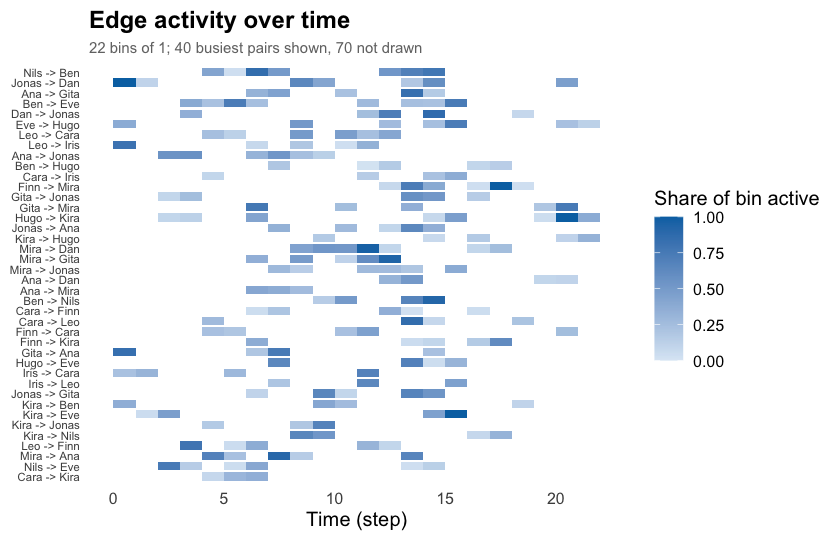
The timeline plot displays when each pair of vertices is connected during the observation period. For interval data, colour indicates the proportion of each time bin during which at least one relational spell is active. Overlapping spells between the same endpoints are counted once, so the plot represents the duration of connectivity rather than the number of interactions.
plot(dn)
Window-based analyses use four arguments to define when measurements
are taken and which interactions they include. start and
end delimit the measurement period. step
specifies the interval between measurements, while window
specifies the duration covered by each measurement. Setting
window equal to step produces non-overlapping
intervals; a larger window produces overlapping intervals.
For snapshot measures, window = 0 evaluates the network at
individual time points.
metrics() computes graph-level measures within the
specified temporal windows. These measures describe the structure of the
network as a whole. For example, density is the proportion of possible
ties present within a window, while reciprocity describes the extent to
which directed ties are reciprocated. Other measures characterise
connected components, local configurations of ties, and the distribution
of centrality across vertices.
The following call computes density at one-unit intervals, using a
seven-unit window for each measurement. Because window
exceeds step, successive measurements include overlapping
periods.
density <- metrics(dn, measure = "density", step = 1, window = 7)
density
#> # Density (graph-level)
#> # 22 time points, step 1, window 7 (rolling) | time in step
#>  time measure     value
#>     0 density 0.3241758
#>     1 density 0.3461538
#>     2 density 0.3571429
#>     3 density 0.3791209
#>     4 density 0.3681319
#>     5 density 0.3791209
#>     6 density 0.3791209
#>     7 density 0.3791209
#>     8 density 0.3956044
#>     9 density 0.3736264
#>    10 density 0.3626374
#>    11 density 0.3351648
#> # 10 more rows. summary() aggregates them; plot() draws them.
The result is a tidy data frame identifying the measurement time,
measure, and value. Multiple statistics can be requested through
measure; their results are distinguished by the
measure column. Available measures include density,
reciprocity, transitivity, dyad and triad censuses, component counts,
centralisation, and Krackhardt’s indices. Their definitions and
calculation conventions are documented in ?metrics.
summary() summarises the resulting time series,
including its mean, dispersion, range, and peak time.
plot() displays how the measure changes over the
observation period.
summary(density)
#>   measure  n     mean       sd        min       max peak_time
#> 1 density 22 0.285964 0.111584 0.03296703 0.3956044         8
plot(density)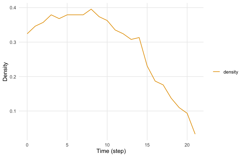
centrality_series() computes measures that describe how
a vertex is connected to the rest of the network. Each centrality
captures a different aspect of structural position.
Degree counts direct connections, indicating the extent
of a vertex’s immediate neighbourhood. In directed networks, indegree
counts incoming connections and outdegree counts outgoing connections.
Strength accounts for the weights of those connections,
distinguishing the number of connected neighbours from the multiplicity
of their relationships.
Closeness centrality is based on the shortest-path distances from a vertex to other vertices. Higher closeness indicates shorter average distances, meaning that fewer steps are required to reach other vertices. In a directed network, these paths follow tie direction.
Betweenness measures the extent to which a vertex lies on shortest paths between other vertices. It therefore identifies potential intermediary positions, although occupying such a position does not establish that information actually passed through that vertex.
Other measures incorporate the positions of a vertex’s neighbours. Eigenvector centrality assigns higher scores to vertices connected to other highly central vertices. PageRank and hub and authority scores also use neighbouring vertices’ scores but apply different rules for directed relationships. Prestige measures characterise a vertex through its incoming connections, including, for some variants, the vertices that can reach it indirectly. The choice of measure should therefore follow the substantive question and the meaning assigned to tie direction.
By default, these measures are calculated within successive temporal windows. This produces a centrality trajectory for each vertex, showing when it becomes more or less connected, accessible, or prominent as an intermediary. The following call computes degree using the default measurement intervals:
degree <- centrality_series(dn, measure = "degree")
degree
#> # Degree (node-level)
#> # 14 vertices | 22 time points, 1 per bin | time in step
#>  time  node measure value
#>     0   Ana  degree     1
#>     0   Ben  degree     1
#>     0  Cara  degree     1
#>     0   Dan  degree     1
#>     0   Eve  degree     2
#>     0  Finn  degree     1
#>     0  Gita  degree     1
#>     0  Hugo  degree     1
#>     0  Iris  degree     2
#>     0 Jonas  degree     2
#>     0  Kira  degree     2
#>     0   Leo  degree     2
#> # 296 more rows. summary() aggregates them; plot() draws them.
The result is a tidy data frame containing vertex names, measurement
times, measures, and values. summary() summarises each
trajectory; peak_time identifies when the corresponding
centrality attained its maximum.
summary(degree)
#>     node measure  n     mean       sd min max peak_time
#> 1    Ana  degree 22 2.181818 2.015095   0   7         6
#> 2    Ben  degree 22 2.000000 1.234427   0   4         4
#> 3   Cara  degree 22 2.227273 1.342770   0   5         4
#> 4    Dan  degree 22 2.090909 1.444500   1   5        13
#> 5    Eve  degree 22 2.272727 2.051290   0   8        14
#> 6   Finn  degree 22 2.000000 1.661898   0   6        12
#> 7   Gita  degree 22 1.727273 1.777688   0   7         6
#> 8   Hugo  degree 22 2.318182 1.861550   0   6         6
#> 9   Iris  degree 22 1.772727 1.066004   0   4        11
#> 10 Jonas  degree 22 2.863636 2.076982   0   7        13
#> 11  Kira  degree 22 2.636364 1.255292   1   6         6
#> 12   Leo  degree 22 1.636364 1.432462   0   5         6
#> 13  Mira  degree 22 2.272727 1.695423   0   6        13
#> 14  Nils  degree 22 2.181818 2.174229   0   7        14
path_centrality() instead computes centrality from
time-respecting paths across the specified observation period.
Temporal closeness measures how quickly a vertex can
reach other reachable vertices, using the inverse of their mean arrival
latency. Temporal betweenness measures a vertex’s
contribution as an intermediary on optimal temporal paths between other
vertices. These measures account for the order and availability of
interactions, whereas window-based centralities describe the connections
present within each window.
closeness <- path_centrality(dn, measure = "closeness")
closeness
#> # Closeness (node-level)
#> # 14 vertices | time in step
#> # computed on time-respecting paths across the whole window
#>   node   measure     value
#>    Ana closeness 0.1313662
#>    Ben closeness 0.1815896
#>   Cara closeness 0.1931075
#>    Dan closeness 0.2230994
#>    Eve closeness 0.2616221
#>   Finn closeness 0.1644945
#>   Gita closeness 0.1404950
#>   Hugo closeness 0.1878341
#>   Iris closeness 0.2398082
#>  Jonas closeness 0.3674392
#>   Kira closeness 0.2107994
#>    Leo closeness 0.3747478
#> # 2 more rows. summary() aggregates them; plot() draws them.paths() examines how a source vertex can reach other
vertices through a sequence of interactions over time. A path may
involve a direct interaction or several intermediate vertices. Each
interaction must occur when its tie is available, and a vertex cannot
pass something onward before receiving it. Waiting between interactions
is permitted: if A contacts B on Monday and B next contacts C on
Wednesday, a path from A to C can include the intervening wait.
The timing of these interactions determines which path arrives
earliest. Suppose A can contact C directly on Friday, but can reach C
through B on Wednesday. The two-hop path through B arrives earlier than
the direct path. paths() therefore minimises arrival time
first, rather than the number of hops. If several paths arrive equally
early, it retains those with the fewest hops.
The following call searches from Ana, beginning at the
start of the observation period in this example:
from_ana <- paths(dn, from = "Ana")
from_ana
#> # Time-respecting paths from 'Ana', from t = 0
#> # reaches 13 of 13 other vertices | time in step
#>   node reachable arrival_time attained latency n_hops n_paths
#>    Ana      TRUE         0.00     TRUE    0.00      0       1
#>    Ben      TRUE         9.59     TRUE    9.59      3       3
#>   Cara      TRUE         6.67     TRUE    6.67      1       1
#>    Dan      TRUE         7.98     TRUE    7.98      4       1
#>    Eve      TRUE        11.66     TRUE   11.66      4       3
#>   Finn      TRUE         6.96     TRUE    6.96      2       1
#>   Gita      TRUE         6.36     TRUE    6.36      2       1
#>   Hugo      TRUE         7.98     TRUE    7.98      3       1
#>   Iris      TRUE        10.00     TRUE   10.00      3       1
#>  Jonas      TRUE         2.12     TRUE    2.12      1       1
#>   Kira      TRUE         6.12     TRUE    6.12      2       2
#>    Leo      TRUE         9.65     TRUE    9.65      3       1
#> # 2 more rows. summary() aggregates them; plot() draws the tree.
The result describes the optimal paths to each destination.
arrival_time records the earliest time at which the
destination can be reached. latency is the elapsed time
between the search origin and arrival, including any waiting for
subsequent interactions. n_hops records how many ties the
path traverses, while n_paths records how many distinct
paths achieve both the earliest arrival and the minimum hop count. A
destination with n_paths = 0 is unreachable under the
specified temporal constraints.
By default, traversing a tie takes zero time, although a path may
still require waiting for a later interaction. A positive
traversal_time assigns a duration to each traversal,
expressed in the network’s time unit. This is an analytical assumption
that affects arrival times and potentially reachability; it should be
selected according to the process being represented.
summary(from_ana)
#>          property   value
#> 1          source     Ana
#> 2       direction forward
#> 3       reachable      13
#> 4 reachable share       1
#> 5  median latency    7.51
#> 6     max latency   11.66
#> 7     median hops       2
#> 8        max hops       4
The summary describes the reachable set and its path characteristics. These results concern possible routes through the recorded relationships. They do not establish that information, resources, or other content actually travelled along those routes.
Reachability also depends on when the search begins. Starting later excludes earlier contacts that may have connected the source to other vertices. The following call starts at time 18:
from_ana_late <- paths(dn, from = "Ana", start = 18)
summary(from_ana_late)
#>          property   value
#> 1          source     Ana
#> 2       direction forward
#> 3       reachable       5
#> 4 reachable share   0.385
#> 5  median latency    2.43
#> 6     max latency    2.68
#> 7     median hops       2
#> 8        max hops       3
Comparing the two results shows how the timing of participation changes the destinations Ana can reach and the routes available to her. This distinction is lost in a static network, where all recorded connections are available without regard to their timing.
pathways() provides the corresponding vertex sequences,
such as A → B → C, and counts the optimal paths following each sequence.
The path plot displays the routes and their temporal progression.
pathways(dn, from = "Ana")
#> # Time-respecting pathways (5 distinct routes)
#> # 7 optimal routes counted
#>                               route endpoint count     share n_hops
#>  Ana -> Jonas -> Kira -> Ben -> Eve      Eve     3 0.4285714      4
#>                 Ana -> Mira -> Gita     Gita     1 0.1428571      2
#>         Ana -> Cara -> Finn -> Iris     Iris     1 0.1428571      3
#>          Ana -> Cara -> Finn -> Leo      Leo     1 0.1428571      3
#>  Ana -> Cara -> Nils -> Hugo -> Dan      Dan     1 0.1428571      4
#>  arrival_time
#>         11.66
#>          6.36
#>         10.00
#>          9.65
#>          7.98
plot(from_ana)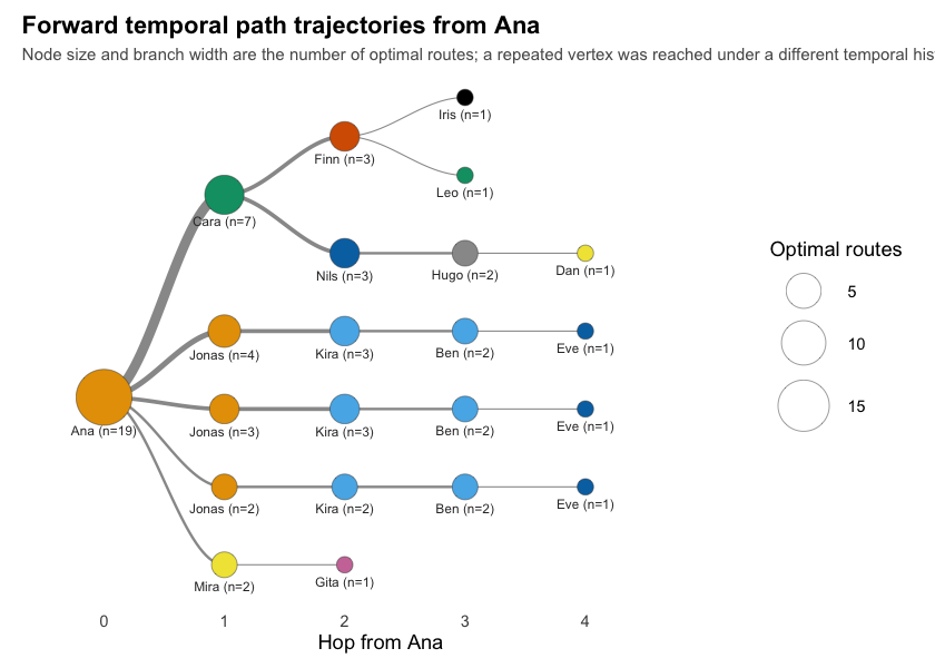
reachability() summarises which vertices can be
connected through time-respecting paths. Forward
reachability identifies the vertices that a source can reach
during the specified observation period. Backward
reachability identifies the vertices from which a focal vertex
can be reached by the end of that period. These sets need not be
identical: the order of interactions may permit a path from A to B
without permitting a return path from B to A.
The direction argument selects "forward",
"backward", or "both". Setting
measure = "reach_count" returns the number of reachable
vertices other than the focal vertex. Setting
measure = "reach" expresses this count as a proportion of
all other vertices in the network.
reach <- reachability(
  dn,
  direction = "both",
  measure = c("reach", "reach_count")
)
reach
#> # Reachability (node-level)
#> # 14 vertices | time in step
#> # measures: forward_reach, forward_reach_count, backward_reach, backward_reach_count
#> # count and share of other vertices joined by a time-respecting path
#>   node       measure value
#>    Ana forward_reach     1
#>    Ben forward_reach     1
#>   Cara forward_reach     1
#>    Dan forward_reach     1
#>    Eve forward_reach     1
#>   Finn forward_reach     1
#>   Gita forward_reach     1
#>   Hugo forward_reach     1
#>   Iris forward_reach     1
#>  Jonas forward_reach     1
#>   Kira forward_reach     1
#>    Leo forward_reach     1
#> # 44 more rows. summary() aggregates them; plot() draws them.
A forward reach of 1 indicates that the source can reach every other vertex within the specified period. A value of 0 indicates that it cannot reach any other vertex. Intermediate values describe partial reachability. These measures include indirect connections through intermediate vertices, so they capture more than the immediate neighbourhood measured by degree.
Reachability describes whether a temporal connection is possible; it does not describe how quickly the destination can be reached. Two vertices can therefore have equal reachability but different temporal closeness because their arrival latencies differ. Examining reachability alongside path timing distinguishes the extent of possible contact from the time required to achieve it.
Relational spells have an onset, a termination, and a duration. Examining these properties describes when relationships become active, when they cease, and how long they persist. In datasets with repeated interactions, several spells may connect the same pair of vertices. Counts of spell onsets and terminations therefore differ from counts of distinct connected pairs.
events() summarises spell onsets and terminations within
temporal windows through the measures "formation" and
"dissolution", which are requested by default. The
following call uses the network’s default measurement intervals:
turnover <- events(dn)
summary(turnover)
#>       measure  n     mean       sd min max peak_time
#> 1 dissolution 22 10.90909 6.132731   3  27        14
#> 2   formation 22 10.90909 6.689787   0  29        13
These counts describe changes in relational activity. A spell onset does not necessarily introduce a previously unconnected pair: it may represent another interaction between endpoints that already have an active spell. Similarly, the termination of one spell does not necessarily disconnect its endpoints if another spell remains active.
durations() summarises the duration of relationships. By
default, results are grouped by endpoint pair. Setting
measure = "mean" returns the mean spell duration for each
pair:
lengths <- durations(dn, measure = "mean")
lengths
#> # Relationship duration (edge-level)
#> # time in step
#> # durations in step
#>  from    to measure     value
#>   Ana  Cara    mean 0.1000000
#>   Ana   Dan    mean 0.3400000
#>   Ana  Gita    mean 0.4220000
#>   Ana  Iris    mean 0.5000000
#>   Ana Jonas    mean 0.5850000
#>   Ana  Kira    mean 0.1100000
#>   Ana   Leo    mean 1.1900000
#>   Ana  Mira    mean 0.3466667
#>   Ben   Eve    mean 0.6100000
#>   Ben  Finn    mean 0.2300000
#>   Ben  Gita    mean 0.3400000
#>   Ben  Hugo    mean 0.1475000
#> # 98 more rows. summary() aggregates them; plot() draws them.
Different duration summaries answer different questions. Summed duration adds the durations of individual spells, including overlapping spells separately. Union duration measures the total time during which at least one spell connects the endpoints, counting overlap once. For example, if two spells connect the same pair during hours 1–3 and 2–4, their summed duration is four hours, while their union duration is three hours. Mean duration describes the average length of an individual spell.
The unit argument determines whether durations are
summarised for endpoint pairs, individual spells, vertex activity, or
ties incident to a vertex. Vertex activity describes when a vertex is
present or eligible to participate; incident-tie duration describes its
recorded relationships. These quantities should be interpreted
separately.
burstiness() describes how interactions are distributed
over time using the intervals between successive events. Regular
activity produces intervals of similar length, whereas clustered
activity produces short intervals within bursts and longer intervals
between them. The burstiness coefficient summarises this variation: −1
corresponds to equal intervals, 0 to the exponential inter-event
distribution associated with a Poisson process, and values approaching 1
indicate increasingly heterogeneous intervals (Goh and Barabási,
2008).
rhythm <- burstiness(dn)
summary(rhythm)
#>     node    measure n        mean sd         min         max
#> 1    Ana burstiness 1  0.24575324 NA  0.24575324  0.24575324
#> 2    Ana     events 1 36.00000000 NA 36.00000000 36.00000000
#> 3    Ana     memory 1 -0.03128243 NA -0.03128243 -0.03128243
#> 4    Ben burstiness 1  0.03288611 NA  0.03288611  0.03288611
#> 5    Ben     events 1 34.00000000 NA 34.00000000 34.00000000
#> 6    Ben     memory 1 -0.19926343 NA -0.19926343 -0.19926343
#> 7   Cara burstiness 1 -0.05610924 NA -0.05610924 -0.05610924
#> 8   Cara     events 1 35.00000000 NA 35.00000000 35.00000000
#> 9   Cara     memory 1  0.07458054 NA  0.07458054  0.07458054
#> 10   Dan burstiness 1 -0.05061772 NA -0.05061772 -0.05061772
#> 11   Dan     events 1 35.00000000 NA 35.00000000 35.00000000
#> 12   Dan     memory 1  0.21654310 NA  0.21654310  0.21654310
#> 13   Eve burstiness 1  0.09217906 NA  0.09217906  0.09217906
#> 14   Eve     events 1 34.00000000 NA 34.00000000 34.00000000
#> 15   Eve     memory 1  0.25882509 NA  0.25882509  0.25882509
#> 16  Finn burstiness 1  0.02938507 NA  0.02938507  0.02938507
#> 17  Finn     events 1 29.00000000 NA 29.00000000 29.00000000
#> 18  Finn     memory 1 -0.22653754 NA -0.22653754 -0.22653754
#> 19  Gita burstiness 1  0.06104200 NA  0.06104200  0.06104200
#> 20  Gita     events 1 31.00000000 NA 31.00000000 31.00000000
#> 21  Gita     memory 1  0.21165690 NA  0.21165690  0.21165690
#> 22  Hugo burstiness 1  0.09885443 NA  0.09885443  0.09885443
#> 23  Hugo     events 1 34.00000000 NA 34.00000000 34.00000000
#> 24  Hugo     memory 1  0.11283700 NA  0.11283700  0.11283700
#> 25  Iris burstiness 1 -0.05968068 NA -0.05968068 -0.05968068
#> 26  Iris     events 1 30.00000000 NA 30.00000000 30.00000000
#> 27  Iris     memory 1 -0.09356972 NA -0.09356972 -0.09356972
#> 28 Jonas burstiness 1 -0.02750549 NA -0.02750549 -0.02750549
#> 29 Jonas     events 1 46.00000000 NA 46.00000000 46.00000000
#> 30 Jonas     memory 1  0.23391957 NA  0.23391957  0.23391957
#> 31  Kira burstiness 1 -0.07048265 NA -0.07048265 -0.07048265
#> 32  Kira     events 1 38.00000000 NA 38.00000000 38.00000000
#> 33  Kira     memory 1 -0.14972726 NA -0.14972726 -0.14972726
#> 34   Leo burstiness 1 -0.01020265 NA -0.01020265 -0.01020265
#> 35   Leo     events 1 28.00000000 NA 28.00000000 28.00000000
#> 36   Leo     memory 1  0.48001912 NA  0.48001912  0.48001912
#> 37  Mira burstiness 1  0.09968547 NA  0.09968547  0.09968547
#> 38  Mira     events 1 36.00000000 NA 36.00000000 36.00000000
#> 39  Mira     memory 1  0.18691159 NA  0.18691159  0.18691159
#> 40  Nils burstiness 1  0.08408761 NA  0.08408761  0.08408761
#> 41  Nils     events 1 34.00000000 NA 34.00000000 34.00000000
#> 42  Nils     memory 1  0.22784733 NA  0.22784733  0.22784733
Burstiness and memory describe different properties of event timing. Burstiness measures variation in interval lengths, without considering their order. Memory measures the correlation between consecutive intervals. Positive memory indicates that short intervals tend to follow short intervals and long intervals tend to follow long intervals. Negative memory indicates a tendency for short and long intervals to alternate. A value near zero indicates little linear association between successive intervals.
A vertex can therefore exhibit bursty activity without substantial memory: its inter-event intervals may vary considerably while consecutive interval lengths remain weakly correlated. Interpreting both measures helps distinguish variability in activity timing from dependence between successive intervals.
mixing() counts distinct active vertex pairs within and
between groups defined by a vertex attribute. Repeated spells and their
weights do not multiply these binary-dyad counts. The forum network
inherits role from forum_people. Setting
step = 60, which exceeds this network’s observation period,
produces a single interval for the comparison.
mixing(forum, attribute = "role", step = 60)
#> # Mixing by role (graph-level)
#> # 1 time points, 60 per bin | time in days
#> # measures: Facilitator -> Facilitator, Student -> Facilitator, Teacher -> Facilitator, Facilitator -> Student, Student -> Student, Teacher -> Student, Facilitator -> Teacher, Student -> Teacher, Teacher -> Teacher
#> # active binary-dyad counts between vertex groups per time bin
#>  time                    measure value  from_group    to_group
#>     0 Facilitator -> Facilitator     0 Facilitator Facilitator
#>     0     Student -> Facilitator     3     Student Facilitator
#>     0     Teacher -> Facilitator     0     Teacher Facilitator
#>     0     Facilitator -> Student     4 Facilitator     Student
#>     0         Student -> Student   136     Student     Student
#>     0         Teacher -> Student    12     Teacher     Student
#>     0     Facilitator -> Teacher     1 Facilitator     Teacher
#>     0         Student -> Teacher    16     Student     Teacher
#> 0 Teacher -> Teacher 0 Teacher Teachercollapse_network() summarises a temporal network as a
weighted static network. Each edge represents a pair of vertices
connected during the observation period, and its weight summarises their
relational spells according to the selected rule. This provides an
overall description of relationships while removing their temporal
order.
Setting weight = "union_duration" assigns each edge the
total time during which at least one spell connects its endpoints.
Overlapping spells are counted once. For example, spells spanning hours
1–3 and 2–4 produce an edge weight of three hours.
flat <- collapse_network(dn, weight = "union_duration")
flat
#> # Collapsed temporal network | 14 vertices | 110 edges | weight: union_duration
#> # 0 to 21.52 step
#>  from    to binary union_duration total_duration duration_fraction spell_count
#>   Ana  Cara      1           0.10           0.10       0.004646840           1
#>   Ana   Dan      1           1.02           1.02       0.047397770           3
#>   Ana  Gita      1           1.99           2.11       0.092472119           5
#>   Ana  Iris      1           0.50           0.50       0.023234201           1
#>   Ana Jonas      1           2.34           2.34       0.108736059           4
#>   Ana  Kira      1           0.11           0.11       0.005111524           1
#>  weight_sum weighted_duration latest_weight first  last activity.duration
#>           1              0.10             1  6.67  6.77              0.10
#>           3              1.02             1 12.04 20.10              1.02
#>           5              2.11             1  6.57 14.16              1.99
#>           1              0.50             1 13.80 14.30              0.50
#>           4              2.34             1  2.12  9.13              2.34
#>           1              0.11             1 11.60 11.71              0.11
#>  activity.count
#>               1
#>               3
#>               5
#>               1
#>               4
#>               1
induce_subgraph() selects part of the network for
further analysis. Selection may be based on vertex attributes or
structural measures. In the following example, degree is calculated over
the full observation period, and vertices with degree greater than 16
are retained together with the relational spells connecting them.
core <- induce_subgraph(dn, degree > 16)
core
#> # Temporal network (interval format, directed) | a cograph netobject
#> # 5 vertices | 31 edge spells | 14 distinct pairs
#> # observed from 0 to 20.46 step, binned every 1
#>
#>   from    to start  end duration weight
#>  Jonas   Dan  0.00 1.10     1.10      1
#>    Eve  Kira  0.77 1.42     0.65      1
#>   Kira   Eve  1.95 2.47     0.52      1
#>  Jonas  Kira  2.05 2.09     0.04      1
#>    Dan Jonas  3.14 3.49     0.35      1
#>    Dan   Eve  3.20 3.33     0.13      1
#> # 25 more spells. summary() describes the network; plot() draws it.
snapshots() extracts connections within specified
temporal windows. The following call returns the connections in the
default measurement window containing time 3:
snapshots(dn, at = 3)
#> # Snapshot edges | 1 bin | 12 tie rows | time in step
#>    time from    to weight n_spells
#> 1     3  Ana Jonas      1        1
#> 2     3 Kira   Leo      1        1
#> 3     3  Leo  Finn      1        1
#> 4     3 Nils   Eve      1        1
#> 5     3  Ben Jonas      1        1
#> 6     3  Ben   Eve      1        1
#> 7     3  Dan   Ana      1        1
#> 8     3  Dan Jonas      1        1
#> 9     3  Dan   Eve      1        1
#> 10    3 Gita Jonas      1        1
#> # 2 more rows. summary() counts them by bin.
A snapshot summarises connectivity within its window; it does not retain the ordering of interactions within that interval.
Dynet provides functions for modifying vertices, relational spells, and observation settings. Each editing function returns a modified network without changing the input object. This allows alternative network specifications to be constructed while retaining the original for comparison.
add_nodes() adds vertices and their attributes.
add_ties() adds relational spells using their endpoints,
onset, and termination. The following example adds a vertex named
Omar, then adds a directed relationship from
Ana to Omar, active from time 4 to time 6:
dn2 <- add_nodes(dn, data.frame(name = "Omar"))
dn2 <- add_ties(dn2, data.frame(from = "Ana", to = "Omar", start = 4, end = 6))
dn2
#> # Temporal network (interval format, directed) | a cograph netobject
#> # 15 vertices | 241 edge spells | 111 distinct pairs
#> # observed from 0 to 21.52 step, binned every 1
#>
#>   from   to start  end duration weight
#>  Jonas  Dan  0.00 1.10     1.10      1
#>   Gita  Ana  0.14 0.98     0.84      1
#>    Leo Mira  0.15 0.42     0.27      1
#>    Leo Iris  0.15 0.96     0.81      1
#>   Kira  Ben  0.33 0.69     0.36      1
#>    Leo Iris  0.38 0.50     0.12      1
#> # 235 more spells. summary() describes the network; plot() draws it.
Related functions support removal, revision, and relabelling.
remove_nodes() and remove_ties() remove
selected vertices or spells; update_nodes() and
update_ties() revise their attributes or values; and
rename_nodes() changes vertex names while maintaining their
references in the network.
set_vertex_spells() specifies periods during which
vertices are present or eligible to participate.
set_observations() specifies the periods over which the
network is observed. These declarations serve different purposes: vertex
activity constrains participation, whereas observation periods constrain
measurement. Changing observation settings does not alter the original
relational spell endpoints.
Temporal network visualisations describe both the structure of relationships and their development over time. Different views address different questions: which vertices are connected during a particular period, how connectivity changes between periods, and when individual relationships are active.
Setting type = "network" displays connections within a
selected measurement window. The at argument identifies the
time of interest. Setting type = "snapshots" displays
several temporal slices using a shared layout, making changes in
connections easier to compare.
plot(dn, type = "network", at = 3)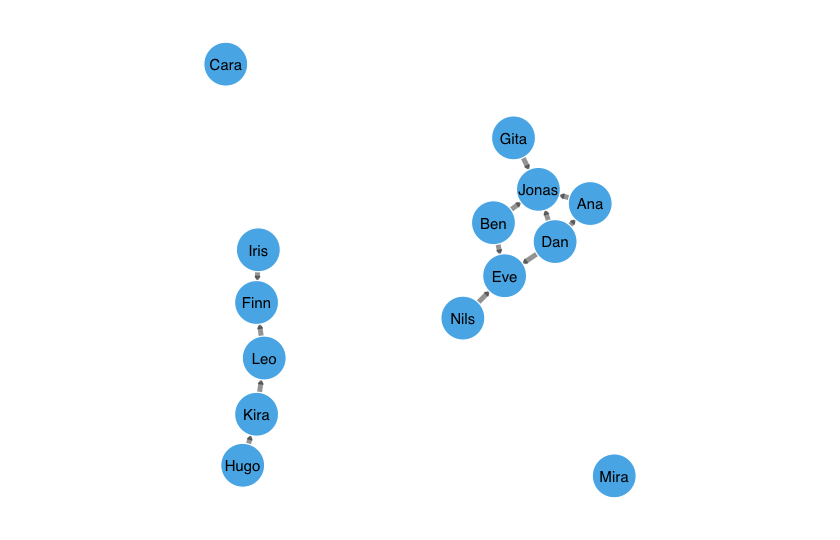
plot(dn, type = "snapshots", panels = 6)
#> Drawing 6 of 22 bins, evenly spaced across the window.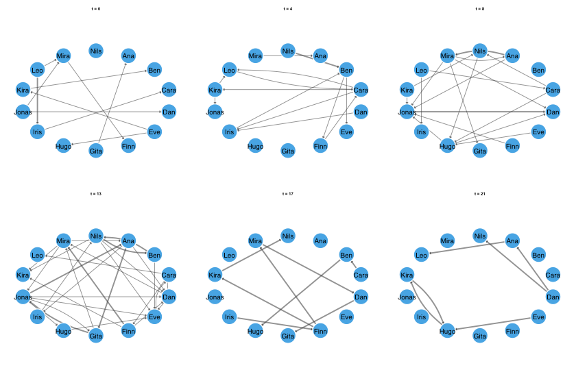
A timeline places relational activity along a time axis. For interval data, colour represents the proportion of each time bin during which an endpoint pair is connected. This view shows periods of activity and inactivity that may be difficult to distinguish in successive network diagrams.
plot(dn, type = "timeline")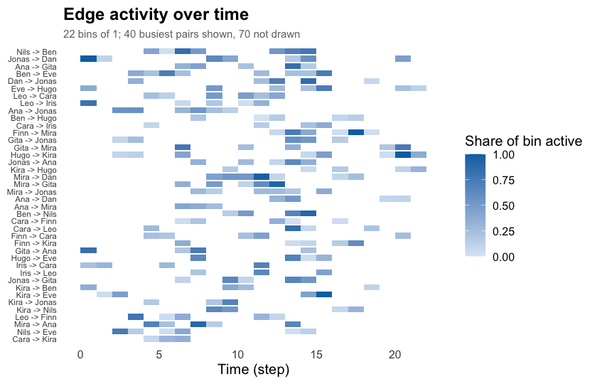
A proximity timeline follows the changing relationships among vertices. Network distances are calculated within temporal slices and represented as positions along a single axis. Lines connect each vertex’s positions across slices, showing how its proximity to other vertices changes. Nearby lines indicate shorter network distances in the corresponding slice; they do not necessarily indicate a direct tie.
plot(dn, type = "proximity")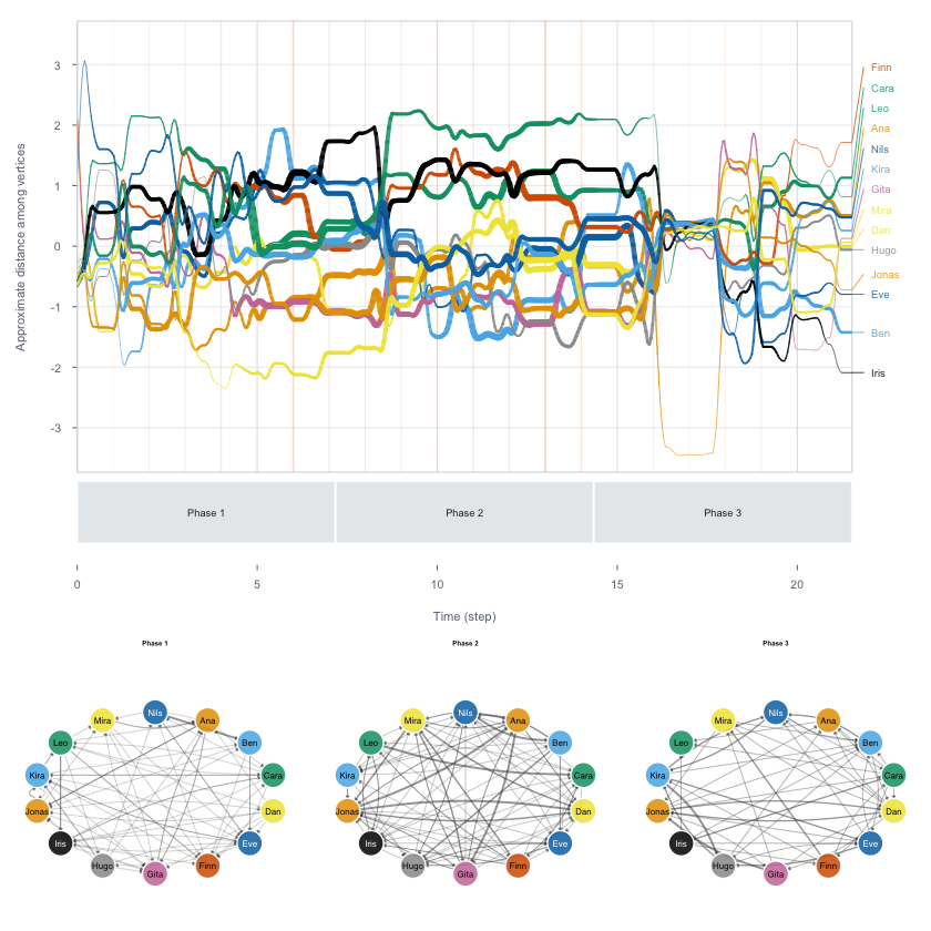
These views complement one another: network diagrams show connections, activity timelines show their timing, and proximity timelines summarise changes in network distances.
animate() displays a sequence of network snapshots over
the observation period. Vertices retain a shared layout across frames,
allowing changes in connections to be followed without changes in
position obscuring the comparison.
The temporal settings follow the same conventions as window-based
measurement. start and end delimit the period,
step determines the time between successive frames, and
window determines the period represented in each frame. A
positive window displays connections active within that interval; it
does not imply that all displayed connections were active
simultaneously.
The output filename determines the format. GIF output requires the
gifski package, while MP4 and WebM output require
av. The animation tutorial provides examples of temporal
settings, visual options, and export procedures.
The package documentation provides additional examples and methodological details:
vignette("dynet") presents an analysis from network
construction through measurement and interpretation.vignette("building-networks") explains input formats,
column recognition, vertex attributes, observation periods, sessions,
and censoring.vignette("ch17-temporal-networks") reproduces the
temporal network analysis chapter of Learning Analytics Methods and
Tutorials using the bundled MOOC data.thought_chains.Function help pages document arguments, defaults, return values, and
calculation conventions. For example, ?dynet,
?metrics, and ?paths describe network
construction, graph-level measurement, and temporal path analysis,
respectively.
Butts, C. T. (2008). A relational event framework for social action. Sociological Methodology, 38(1), 155–200.
Goh, K.-I., & Barabási, A.-L. (2008). Burstiness and memory in complex systems. EPL (Europhysics Letters), 81(4), 48002.
Holme, P., & Saramäki, J. (2012). Temporal networks. Physics Reports, 519(3), 97–125.
Kempe, D., Kleinberg, J., & Kumar, A. (2002). Connectivity and inference problems for temporal networks. Journal of Computer and System Sciences, 64(4), 820–842.
Masuda, N., & Lambiotte, R. (2016). A guide to temporal networks. World Scientific.
Moody, J. (2002). The importance of relationship timing for diffusion. Social Forces, 81(1), 25–56.
Nicosia, V., Tang, J., Mascolo, C., Musolesi, M., Russo, G., & Latora, V. (2013). Graph metrics for temporal networks. In P. Holme & J. Saramäki (Eds.), Temporal networks (pp. 15–40). Springer.
Pan, R. K., & Saramäki, J. (2011). Path lengths, correlations, and centrality in temporal networks. Physical Review E, 84(1), 016105.
Saqr, M. (2024). Temporal network analysis: Introduction, methods and analysis with R. In M. Saqr & S. López-Pernas (Eds.), Learning analytics methods and tutorials: A practical guide using R. Springer.
Saqr, M., López-Pernas, S., & Törmänen, T. (2026). A temporal network approach to reveal the longitudinal dynamics of CSCL group regulation and productive collaboration. International Journal of Computer-Supported Collaborative Learning, 21, 237–270. https://doi.org/10.1007/s11412-025-09464-5
Saqr, M., & Nouri, J. (2020). High resolution temporal network analysis to understand and improve collaborative learning. In Proceedings of the Tenth International Conference on Learning Analytics & Knowledge (pp. 314–319). ACM.
Saqr, M., & Peeters, W. (2022). Temporal networks in collaborative learning: A case study. British Journal of Educational Technology, 53(5), 1283–1303. https://doi.org/10.1111/bjet.13187
These binaries (installable software) and packages are in development.
They may not be fully stable and should be used with caution. We make no claims about them.