The hardware and bandwidth for this mirror is donated by METANET, the Webhosting and Full Service-Cloud Provider.
If you wish to report a bug, or if you are interested in having us mirror your free-software or open-source project, please feel free to contact us at mirror[@]metanet.ch.
![]()
![]()
![]()
The goal of the LMMsolver package is to fit
(generalized) linear mixed models efficiently when the model structure
is large or sparse. It provides tools for estimating variance components
using restricted maximum likelihood (REML) and is designed for models
that involve many random effects or smooth terms.
A key feature of the package is support for smoothing using P-splines. LMMsolver uses a sparse formulation (Boer 2023), which makes computations fast and memory efficient, especially for two-dimensional smoothing problems such as spatial surfaces or image-like data (Boer 2023; Carollo et al. 2024).
This makes LMMsolver particularly useful for
applications involving spatial or temporal smoothing, large data sets,
and models where standard mixed model tools become slow or
impractical.
install.packages("LMMsolver")remotes::install_github("Biometris/LMMsolver", ref = "develop", dependencies = TRUE)As an example of the functionality of the package we use the
USprecip data set in the spam package (Furrer
and Sain 2010).
library(LMMsolver)
library(ggplot2)

## Get precipitation data from spam
data(USprecip, package = "spam")

## Only use observed data.
USprecip <- as.data.frame(USprecip)
USprecip <- USprecip[USprecip$infill == 1, ]
head(USprecip[, c(1, 2, 4)], 3)
#>      lon   lat  anomaly
#> 6 -85.95 32.95 -0.84035
#> 7 -85.87 32.98 -0.65922
#> 9 -88.28 33.23 -0.28018
A two-dimensional P-spline can be defined with the
spl2D() function, with longitude and latitude as
covariates, and anomaly (standardized monthly total precipitation) as
response variable:
obj1 <- LMMsolve(fixed = anomaly ~ 1,
                 spline = ~spl2D(x1 = lon, x2 = lat, nseg = c(41, 41)),
                 data = USprecip)
The spatial trend for the precipitation can now be plotted on the map
of the USA, using the predict function of
LMMsolver:
newdat <- makeGrid(obj1, grid = c(200, 300))
plotDat <- predict(obj1, newdata = newdat)

plotDat <- sf::st_as_sf(plotDat, coords = c("lon", "lat"))
usa <- sf::st_as_sf(maps::map("usa", regions = "main", plot = FALSE))
sf::st_crs(usa) <- sf::st_crs(plotDat)
intersection <- sf::st_intersects(plotDat, usa)
plotDat <- plotDat[!is.na(as.numeric(intersection)), ]

ggplot(usa) +
  geom_sf(color = NA) +
  geom_tile(data = plotDat,
            mapping = aes(geometry = geometry, fill = ypred),
            linewidth = 0,
            stat = "sf_coordinates") +
  scale_fill_gradientn(colors = topo.colors(100))+
  labs(title = "Precipitation (anomaly)",
       x = "Longitude", y = "Latitude") +
  coord_sf() +
  theme(panel.grid = element_blank())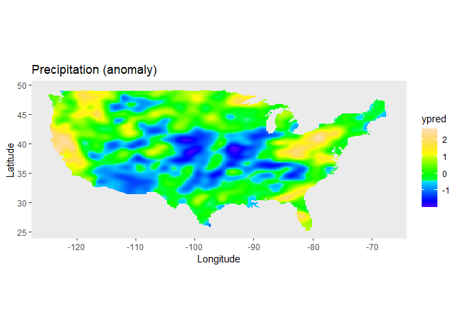
Further examples can be found in the vignette.
vignette("Solving_Linear_Mixed_Models")These binaries (installable software) and packages are in development.
They may not be fully stable and should be used with caution. We make no claims about them.