The hardware and bandwidth for this mirror is donated by METANET, the Webhosting and Full Service-Cloud Provider.
If you wish to report a bug, or if you are interested in having us mirror your free-software or open-source project, please feel free to contact us at mirror[@]metanet.ch.
A number of utilities for dealing with the Markowitz portfolio.
– Steven E. Pav, shabbychef@gmail.com
This package may be installed from CRAN; the latest version may be found on github via devtools:
if (require(devtools)) {
    # latest greatest
    install_github(repo = "MarkowitzR", username = "shabbychef",
        ref = "master")
}The (negative) Markowitz portfolio appears in the inverse of the uncentered second moment matrix of the ‘augmented’ vector of returns. Via the Central Limit Theorem and the delta method the asymptotic distribution of the Markowitz portfolio can be found. From this, Wald statistics on the individual portfolio weights can be computed.
First for unconditional returns:
set.seed(1001)
X <- matrix(rnorm(1000 * 3), ncol = 3)
ism <- mp_vcov(X, fit.intercept = TRUE)
walds <- ism$W/sqrt(diag(ism$What))
print(t(walds))
## X1 X2 X3
## Intercept 0.83 -0.15 -1.8Now for conditional expectation:
# generate data with given W, Sigma
Xgen <- function(W, Sigma, Feat) {
    Btrue <- Sigma %*% W
    Xmean <- Feat %*% t(Btrue)
    Shalf <- chol(Sigma)
    X <- Xmean + matrix(rnorm(prod(dim(Xmean))), ncol = dim(Xmean)[2]) %*%
        Shalf
}

n.feat <- 3
n.ret <- 5
n.obs <- 2000
set.seed(101)
Feat <- matrix(rnorm(n.obs * n.feat), ncol = n.feat)
Wtrue <- 5 * matrix(rnorm(n.feat * n.ret), ncol = n.feat)
Sigma <- cov(matrix(rnorm(100 * n.ret), ncol = n.ret))
Sigma <- Sigma + diag(seq(from = 1, to = 3, length.out = n.ret))
X <- Xgen(Wtrue, Sigma, Feat)
ism <- mp_vcov(X, feat = Feat, fit.intercept = TRUE)

walds <- ism$W/sqrt(diag(ism$What))
print(t(walds))
## X1 X2 X3 X4 X5
## Intercept -0.61 0.4 0.11 0.61 0.2
## Feat1 0.30 -20.7 14.56 -10.70 -24.6
## Feat2 -14.82 -4.0 12.01 29.75 -1.8
## Feat3 16.62 -5.3 -30.41 0.83 3.5# results are not much changed when using robust
# s.e.
library(sandwich)
ism.rse <- mp_vcov(X, feat = Feat, vcov.func = sandwich::vcovHAC,
fit.intercept = TRUE)
walds.rse <- ism.rse$W/sqrt(diag(ism.rse$What))
print(t(walds.rse))## X1 X2 X3 X4 X5
## Intercept -0.61 0.4 0.11 0.60 0.19
## Feat1 0.29 -20.4 14.43 -10.66 -24.45
## Feat2 -14.49 -3.9 11.88 29.60 -1.80
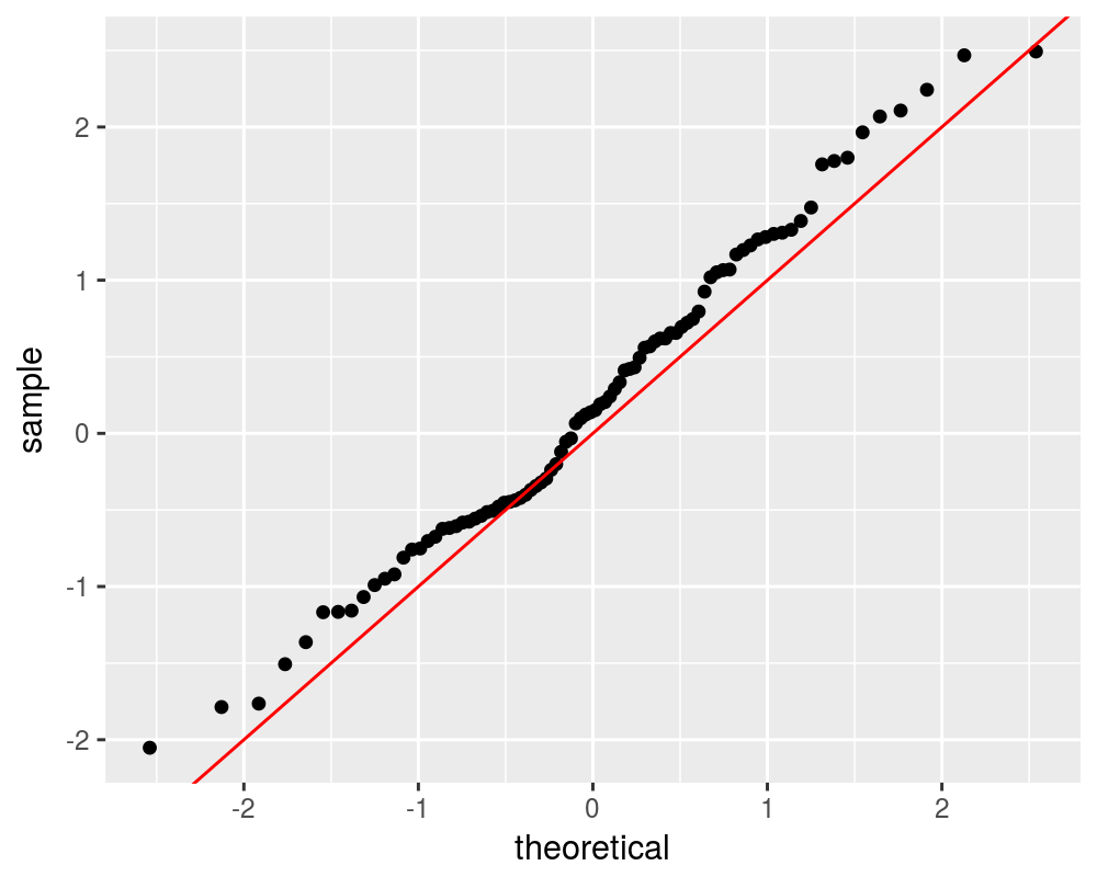
## Feat3 16.37 -5.3 -29.85 0.83 3.48# errors should be asymptotically normal with the
# given covariance.
n.feat <- 5
n.ret <- 15
n.obs <- 3000
set.seed(101)
Feat <- matrix(rnorm(n.obs * n.feat), ncol = n.feat)
Wtrue <- 5 * matrix(rnorm(n.feat * n.ret), ncol = n.feat)
Sigma <- cov(matrix(rnorm(100 * n.ret), ncol = n.ret))
Sigma <- Sigma + diag(seq(from = 1, to = 3, length.out = n.ret))
X <- Xgen(Wtrue, Sigma, Feat)
ism <- mp_vcov(X, feat = Feat, fit.intercept = TRUE)
Wcomp <- cbind(0, Wtrue)
errs <- ism$W - Wcomp
dim(errs) <- c(length(errs), 1)
Zerr <- solve(t(chol(ism$What)), errs)
print(summary(Zerr))## V1
## Min. :-2.05
## 1st Qu.:-0.55
## Median : 0.14
## Mean : 0.20
## 3rd Qu.: 1.00
## Max. : 2.49library(ggplot2)
ph <- ggplot(data.frame(Ze = Zerr), aes(sample = Ze)) +
stat_qq() + geom_abline(slope = 1, intercept = 0,
colour = "red")
print(ph)
# qqnorm(Zerr) qqline(Zerr,col=2)Now load the Fama French 3 factor portfolios.
if (!require(aqfb.data, quietly = TRUE) && require(devtools)) {
    # get the 10 industry data
    devtools::install_github("shabbychef/aqfb_data")
}
library(aqfb.data)
# fama
data(mff4)

# will not matter, but convert pcts:
ff.data <- 0.01 * mff4

# risk free rate:
rfr <- ff.data[, "RF"]

# subtract risk free from Mkt, HML and SMB:
ff.ret <- ff.data[, c("Mkt", "HML", "SMB")] - rep(rfr,
    2)
Now analyze the Markowitz portfolio on them.
ism <- mp_vcov(ff.ret, fit.intercept = TRUE)
walds <- ism$W/sqrt(diag(ism$What))
print(t(walds))
## Mkt HML SMB
## Intercept 4 0.32 -2# now consider the hedging constraint: no
# covariance with the market:
Gmat <- matrix(c(1, 0, 0), nrow = 1)
ism <- mp_vcov(ff.ret, fit.intercept = TRUE, Gmat = Gmat)
walds <- ism$W/sqrt(diag(ism$What))
print(t(walds))## Mkt HML SMB
## Intercept 1.5 0.32 -2These binaries (installable software) and packages are in development.
They may not be fully stable and should be used with caution. We make no claims about them.