The hardware and bandwidth for this mirror is donated by METANET, the Webhosting and Full Service-Cloud Provider.
If you wish to report a bug, or if you are interested in having us mirror your free-software or open-source project, please feel free to contact us at mirror[@]metanet.ch.
The goal of MortalityTables is to provide generic base classes and functions to handle all kinds of actuarial actuarial mortality tables (period and cohort life tables). Cohort and static life tables are implemented, observed data can be used, and existing life tables can be blended or extrapolated to derive new tables.
Furthermore, plotting functions are provided for reports and publications.
You can install the development version of MortalityTables from GitHub with:
# install.packages("devtools")
devtools::install_github("kainhofer/MortalityTables")The MortalityTables package provides the mortalityTable
base class and some derived classes to handle different types of
mortality tables (also called life tables), mainly used for life
insurance. Additionally it provides a plot function to compare multiple
life tables either directly using the absolute mortalities in log-linear
plots or using relative mortalities as percentages of a given reference
table.
Provided types of mortality tables are:
Base class
Class mortalityTable
Period life table
Class
mortalityTable.period(ages, deathProbs, ..., baseYear=2000)
Death probabilities observed / predicted for one observation year; No dependency on the bith year is assumed.
Cohort life table using age-specific trends
Class mortalityTable.trendProjection
Death probabilities of a given base year are projected into the
future using age-specific trends \(\lambda_x\). The death probability of an
\(x\)-year old in year
baseYear + n is calculated as: \[q_x^{(baseYear+n)} = q_x^{(baseYear)} \cdot
e^{-n\cdot\lambda_x}\]
Consequently, the death probabilities for a person born in year
YOB can be calculated as \[q_x^{YOB} = q_x^{(base)} \cdot
e^{-(YOB+x-baseYear)\cdot \lambda_x}\]
Class mortalityTable.ageShift
Death probabilities for cohort \(YOB\) are obtained by using death probabilities for cohort \(X\) and modifying the technical age with a birth-year dependent shift: \[q_x^{YOB} = q_{x+shift(YOB)}^{(base)}\]
Class mortalityTable.mixed
Arithmetic mean of two life tables with given weights. This approach is often used to generate unisex life tables by mixing male and female mortalities with given weights (e.g. 70:30 or 40:60)
Cohort life table using age-specific improvement factors
Class mortalityTable.improvementFactors
Project base life table using age-specific improvement factors.
Pension table
Class pensionTable
Four states: active, early retirement / invalidity, old-age pension, death (with optional widow)
All slots describe the corresponding transition probabilities by a
mortalityTable-derived object.
library("MortalityTables")The package provides several real-life life tables published by
census bureaus and actuarial associations around the world. You can use
the function mortalityTables.list to list all available
datasets (if no argument is given) or all datasets that match the given
pattern (wildcard character is *). You can then use
mortalityTables.load to load either one single data set or
all datasets that match the pattern.
# list all datasets for Austria
mortalityTables.list("Austria_*")
#>  [1] "Austria_Annuities"                  "Austria_Annuities_AVOe1996R"
#>  [3] "Austria_Annuities_AVOe2005R"        "Austria_Annuities_EROMF"
#>  [5] "Austria_Annuities_RR67"             "Austria_Census"
#>  [7] "Austria_Endowments_ADSt2426_2Lives" "Austria_PopulationForecast"
#>  [9] "Austria_PopulationMCMC"             "Austria_PopulationObserved"
#> [11] "Austria_VUGesamtbestand_2012-16"

# Load the German annuity table DAV 2004-R
mortalityTables.load("Germany_Annuities_DAV2004R")

# Load all Austrian data sets
mortalityTables.load("Austria_*")
#> Lade nötiges Paket: MortalityLaws
#> Warning: Paket 'MortalityLaws' wurde unter R Version 4.2.3 erstellt
Cohort mortality vectors (for a given birth year) or period death
probabilities (for a given observation year) can be extracted with the
functions periodDeathProbabilities() and
deathProbabilities():
mortalityTables.load("Austria_Annuities")
deathProbabilities(AVOe2005R.male, YOB = 1977, ages = 35:50)
#>  [1] 0.0006467352 0.0006741228 0.0007202125 0.0007820113 0.0008524437
#>  [6] 0.0009260103 0.0009794564 0.0010272832 0.0010731228 0.0011227093
#> [11] 0.0011784509 0.0012409740 0.0013080864 0.0013817843 0.0014633494
#> [16] 0.0015513107
deathProbabilities(AVOe2005R.male, YOB = 2023, ages = 35:50)
#>  [1] 0.0001941029 0.0002041420 0.0002200821 0.0002411616 0.0002653197
#>  [6] 0.0002909132 0.0003106056 0.0003288675 0.0003468281 0.0003663459
#> [11] 0.0003882554 0.0004128296 0.0004394048 0.0004687102 0.0005012581
#> [16] 0.0005366270

periodDeathProbabilities(AVOe2005R.male, Period = 2023, ages = 35:50)
#>  [1] 0.0004718782 0.0005066172 0.0005573996 0.0006231746 0.0006993210
#>  [6] 0.0007819197 0.0008511112 0.0009184673 0.0009869854 0.0010620137
#> [11] 0.0011462722 0.0012409740 0.0013445246 0.0014595263 0.0015880515
#> [16] 0.0017292761
If the mortality table is a cohort table, the trend is used to calculate the death probabilities for the given cohort or calendar year. If the table is a static life table, the period and cohort life tables will be identical. If the table is an observed table (i.e. observed death probabilities for each age and year), the data is extracted from the matrix’ rows/columns or diagonals. In all cases, the user does not have use different methods for different underlying tables.
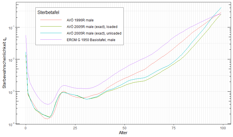
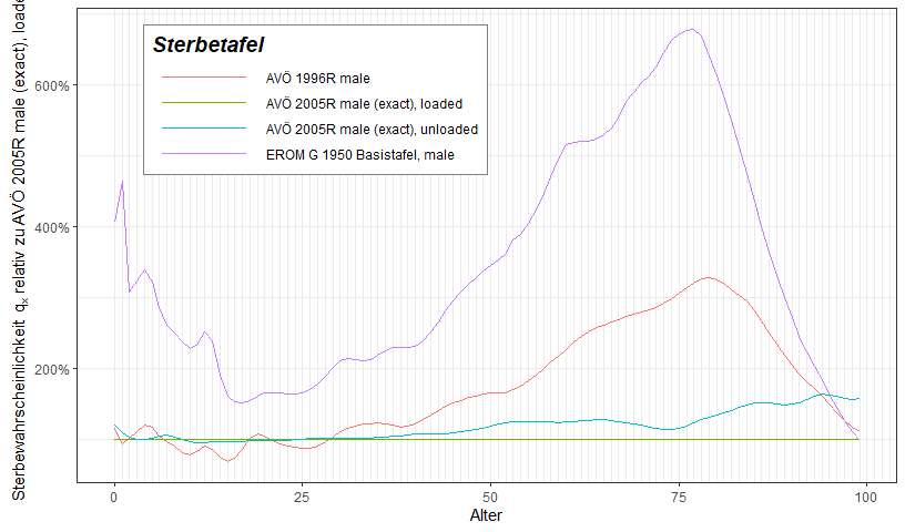
There are two plotting functions using ggplot:
plotMortalityTables() and
plotMortalityTableComparisons() to plot the absolute and
relative mortalities. For absolute mortalities, the q(x)
axis employs a log10-scale. The returned plot is a normal ggplot2
object, so all features provided by ggplot2 can be adde to the
plots.
mortalityTables.load("Austria_Annuities")
plotMortalityTables(AVOe2005R.male, AVOe2005R.male.unloaded, AVOe1996R.male, EROM.G1950.male,
                    YOB = 1977, ages = 0:99, legend.position = c(0.5, 0.65))
plotMortalityTableComparisons(AVOe2005R.male, AVOe2005R.male.unloaded, AVOe1996R.male, EROM.G1950.male,
                              YOB = 1977, ages = 0:99, legend.position = c(0.5, 0.65))
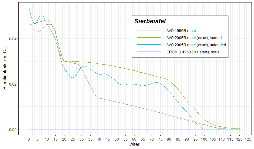
plotMortalityTrend(AVOe2005R.male, AVOe2005R.male.unloaded, AVOe1996R.male, AVOe1996R.male, EROM.G1950.male)
For further information on how to use the package, see the “Using the MortalityTables Package” vignette.
These binaries (installable software) and packages are in development.
They may not be fully stable and should be used with caution. We make no claims about them.