
The hardware and bandwidth for this mirror is donated by METANET, the Webhosting and Full Service-Cloud Provider.
If you wish to report a bug, or if you are interested in having us mirror your free-software or open-source project, please feel free to contact us at mirror[@]metanet.ch.
![]()
This README contains a thorough walkthrough of Bayesian optimization and the syntax needed to use this package, with simple and complex examples. More information can be found in the package vignettes and manual.
You can install the most recent stable version of ParBayesianOptimization from CRAN with:
install.packages("ParBayesianOptimization")You can also install the most recent development version from github using devtools:
# install.packages("devtools")
devtools::install_github("AnotherSamWilson/ParBayesianOptimization")Machine learning projects will commonly require a user to “tune” a model’s hyperparameters to find a good balance between bias and variance. Several tools are available in a data scientist’s toolbox to handle this task, the most blunt of which is a grid search. A grid search gauges the model performance over a pre-defined set of hyperparameters without regard for past performance. As models increase in complexity and training time, grid searches become unwieldly.
Idealy, we would use the information from prior model evaluations to
guide us in our future parameter searches. This is precisely the idea
behind Bayesian Optimization, in which our prior response distribution
is iteratively updated based on our best guess of where the best
parameters are. The ParBayesianOptimization package does
exactly this in the following process:
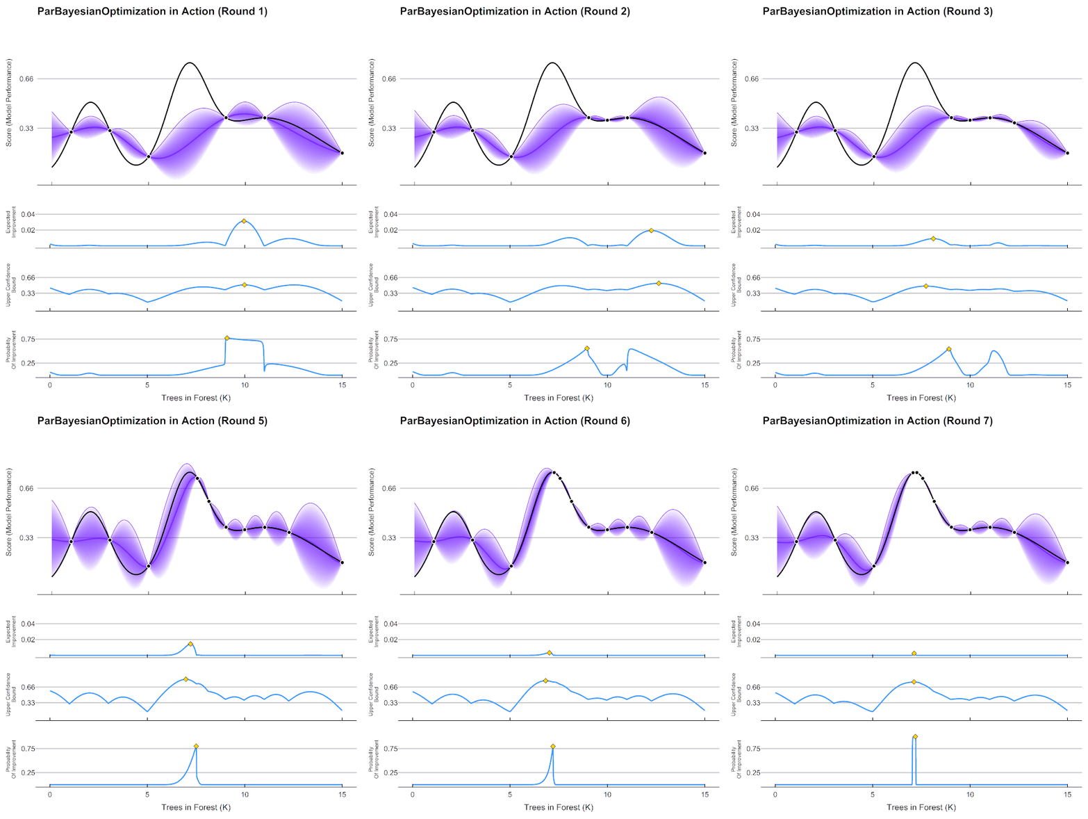
As an example, let’s say we are only tuning 1 hyperparameter in an random forest model, the number of trees, within the bounds [1,15000]. We have initialized the process by randomly sampling the scoring function 7 times, and get the following results:
| Trees.In.Forest | Score |
|---|---|
| 1000 | 0.30 |
| 3000 | 0.31 |
| 5000 | 0.14 |
| 9000 | 0.40 |
| 11000 | 0.40 |
| 15000 | 0.16 |
In this example, Score can be generalized to any error metric that we want to maximize (negative RMSE, AUC, etc.). Keep in mind, Bayesian optimization can be used to maximize any black box function, hyperparameter tuning is just a common use case. Given these scores, how do we go about determining the best number of trees to try next? As it turns out, Gaussian processes can give us a very good definition of our assumption about how the Score (model performance) is distributed over the hyperparameters. Fitting a Gaussian process to the data above, we can see the expected value of Score across our parameter bounds, as well as the uncertainty bands:
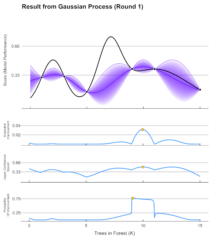
Before we can select our next candidate parameter to run the scoring function on, we need to determine how we define a “good” parameter inside this prior distribution. This is done by maximizing different acquisition functions within the Gaussian process. The acquisition function tells is how much utility there is at a certain unexplored space. In the chart above, the lower 3 graphs show examples different acquisition functions.
Our expected improvement in the graph above is maximized at ~10000.
If we run our process with the new Trees in Forest = 10000,
we can update our Gaussian process for a new prediction about which
would be best to sample next.
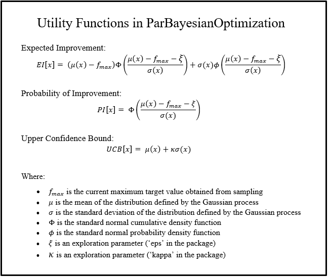
The utility functions that are maximized in this package are defined as follows:
In this example, we are optimizing a simple function with 1 input and 1 output. We, the user, need to define the function that we want to optimize. This function should return, at a minimum, a list with a Score element. You can also return other elements that you want to keep track of in each run of the scoring function, which we show in the section Hyperparameter Tuning.
simpleFunction <- function(x) dnorm(x,3,2)*1.5 + dnorm(x,7,1) + dnorm(x,10,2)

# Find the x that maximizes our simpleFunction
xmax <- optim(8,simpleFunction,method = "L-BFGS-B",lower = 0, upper = 15,control = list(fnscale = -1))$par

# Get a visual
library(ggplot2)
ggplot(data = data.frame(x=c(0,15)),aes(x=x)) +
  stat_function(fun = simpleFunction) +
  geom_vline(xintercept = xmax,linetype="dashed") +
  ggtitle("simpleFunction") +
  theme_bw()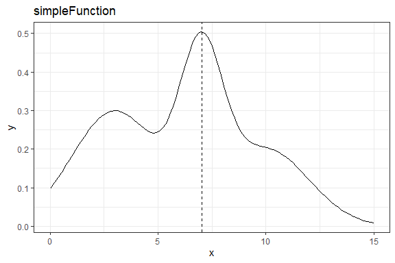
We can see that this function is maximized around x~7.023. We can use
bayesOpt to find the global maximum of this function. We
just need to define the bounds, and the initial parameters we want to
sample:
bounds <- list(x=c(0,15))
initGrid <- data.frame(x=c(0,5,10))
Here, we run bayesOpt. The function begins by running
simpleFunction 3 times, and then fits a Gaussian process to
the results in a process called Kriging. We then
calculate the x which maximizes our expected improvement,
and run simpleFunction at this x. We then go through 1 more
iteration of this:
library(ParBayesianOptimization)

FUN <- function(x) list(Score = simpleFunction(x))

set.seed(6)
optObjSimp <- bayesOpt(
  FUN = FUN
  , bounds = bounds
  , initGrid = initGrid
  , iters.n = 2
)
Let’s see how close the algorithm got to the global maximum:
getBestPars(optObjSimp)
#> $x
#> [1] 6.718184
The process is getting pretty close! We were only about 3% shy of the global optimum:
simpleFunction(getBestPars(optObjSimp)$x)/simpleFunction(7.023)
#> [1] 0.968611
Let’s run the process for a little longer:
optObjSimp <- addIterations(optObjSimp,iters.n=3,verbose=0)
simpleFunction(getBestPars(optObjSimp)$x)/simpleFunction(7.023)
#> [1] 0.9958626
We have now found an x very close to the global
optimum.
In this example, we will be using the agaricus.train dataset provided in the XGBoost package. Here, we load the packages, data, and create a folds object to be used in the scoring function.
library("xgboost")

data(agaricus.train, package = "xgboost")

Folds <- list(
    Fold1 = as.integer(seq(1,nrow(agaricus.train$data),by = 3))
  , Fold2 = as.integer(seq(2,nrow(agaricus.train$data),by = 3))
  , Fold3 = as.integer(seq(3,nrow(agaricus.train$data),by = 3))
)
Now we need to define the scoring function. This function should, at
a minimum, return a list with a Score element, which is the
model evaluation metric we want to maximize. We can also retain other
pieces of information created by the scoring function by including them
as named elements of the returned list. In this case, we want to retain
the optimal number of rounds determined by the xgb.cv:
scoringFunction <- function(max_depth, min_child_weight, subsample) {

  dtrain <- xgb.DMatrix(agaricus.train$data,label = agaricus.train$label)

  Pars <- list(
      booster = "gbtree"
    , eta = 0.001
    , max_depth = max_depth
    , min_child_weight = min_child_weight
    , subsample = subsample
    , objective = "binary:logistic"
    , eval_metric = "auc"
  )

  xgbcv <- xgb.cv(
      params = Pars
    , data = dtrain
    , nround = 100
    , folds = Folds
    , early_stopping_rounds = 5
    , maximize = TRUE
    , verbose = 0
  )

  return(list(Score = max(xgbcv$evaluation_log$test_auc_mean)
             , nrounds = xgbcv$best_iteration
             )
         )
}
We also need to tell our process the bounds it is allowed to search within:
bounds <- list(
    max_depth = c(1L, 5L)
  , min_child_weight = c(0, 25)
  , subsample = c(0.25, 1)
)
We are now ready to put this all into the bayesOpt
function.
set.seed(0)

tNoPar <- system.time(
  optObj <- bayesOpt(
      FUN = scoringFunction
    , bounds = bounds
    , initPoints = 4
    , iters.n = 4
    , iters.k = 1
  )
)
The console informs us that the process initialized by running
scoringFunction 4 times. It then fit a Gaussian process to
the parameter-score pairs, found the global optimum of the acquisition
function, and ran scoringFunction again. This process
continued until we had 6 parameter-score pairs. You can interrogate the
optObj object to see the results:
optObj$scoreSummary
#>    Epoch Iteration max_depth min_child_weight subsample gpUtility acqOptimum inBounds Elapsed     Score nrounds errorMessage
#> 1:     0         1         2         1.670129 0.7880670        NA      FALSE     TRUE    0.14 0.9777163       2           NA
#> 2:     0         2         2        14.913213 0.8763154        NA      FALSE     TRUE    0.33 0.9763760      15           NA
#> 3:     0         3         4        18.833690 0.3403900        NA      FALSE     TRUE    0.43 0.9931657      18           NA
#> 4:     0         4         4         8.639925 0.5499186        NA      FALSE     TRUE    0.23 0.9981437       7           NA
#> 5:     1         5         4        21.871937 1.0000000 0.5857961       TRUE     TRUE    0.12 0.9945933       1           NA
#> 6:     2         6         4         0.000000 0.9439879 0.6668303       TRUE     TRUE    0.25 0.9990567       7           NA
#> 7:     3         7         5         1.395119 0.7071802 0.2973497       TRUE     TRUE    0.18 0.9984577       4           NA
#> 8: 4 8 5 0.000000 0.2500000 0.3221660 TRUE TRUE 0.32 0.9994020 10 NAgetBestPars(optObj)
#> $max_depth
#> [1] 5
#>
#> $min_child_weight
#> [1] 0
#>
#> $subsample
#> [1] 0.25The process that the package uses to run in parallel is explained
above. Actually setting the process up to run in parallel is relatively
simple, we just need to take two extra steps. We need to load any
packages and objects required by FUN into the back ends,
after registering our cluster:
library(doParallel)
cl <- makeCluster(2)
registerDoParallel(cl)
clusterExport(cl,c('Folds','agaricus.train'))
clusterEvalQ(cl,expr= {
  library(xgboost)
})
We can now run our process in paralel! Make sure you set iters.k to
some sensible value to take advantage of the parallelization setup.
Since we have registered 2 cores, we set iters.k to 2:
tWithPar <- system.time(
  optObj <- bayesOpt(
      FUN = scoringFunction
    , bounds = bounds
    , initPoints = 4
    , iters.n = 4
    , iters.k = 2
    , parallel = TRUE
  )
)
stopCluster(cl)
registerDoSEQ()
We managed to massively cut the process time by running the process on 2 cores in parallel. However, keep in mind we only performed 2 optimization steps, versus the 4 performed in the sequential example:
tWithPar
#>    user  system elapsed
#>    0.99    0.03    7.91
tNoPar
#>    user  system elapsed
#> 24.13 2.40 21.70Sometimes we may want to sample multiple promising points at the same
optimization step (Epoch). This is especially effective if the process
is being run in parallel. The bayesOpt function always
samples the global optimum of the acquisition function, however it is
also possible to tell it to sample local optimums of the acquisition
function at the same time.
Using the acqThresh parameter, you can specify the
minimum percentage utility of the global optimum required for a
different local optimum to be considered. As an example, let’s say we
are optimizing 1 input x, which is bounded between [0,1].
Our acquisition function may look like the following:
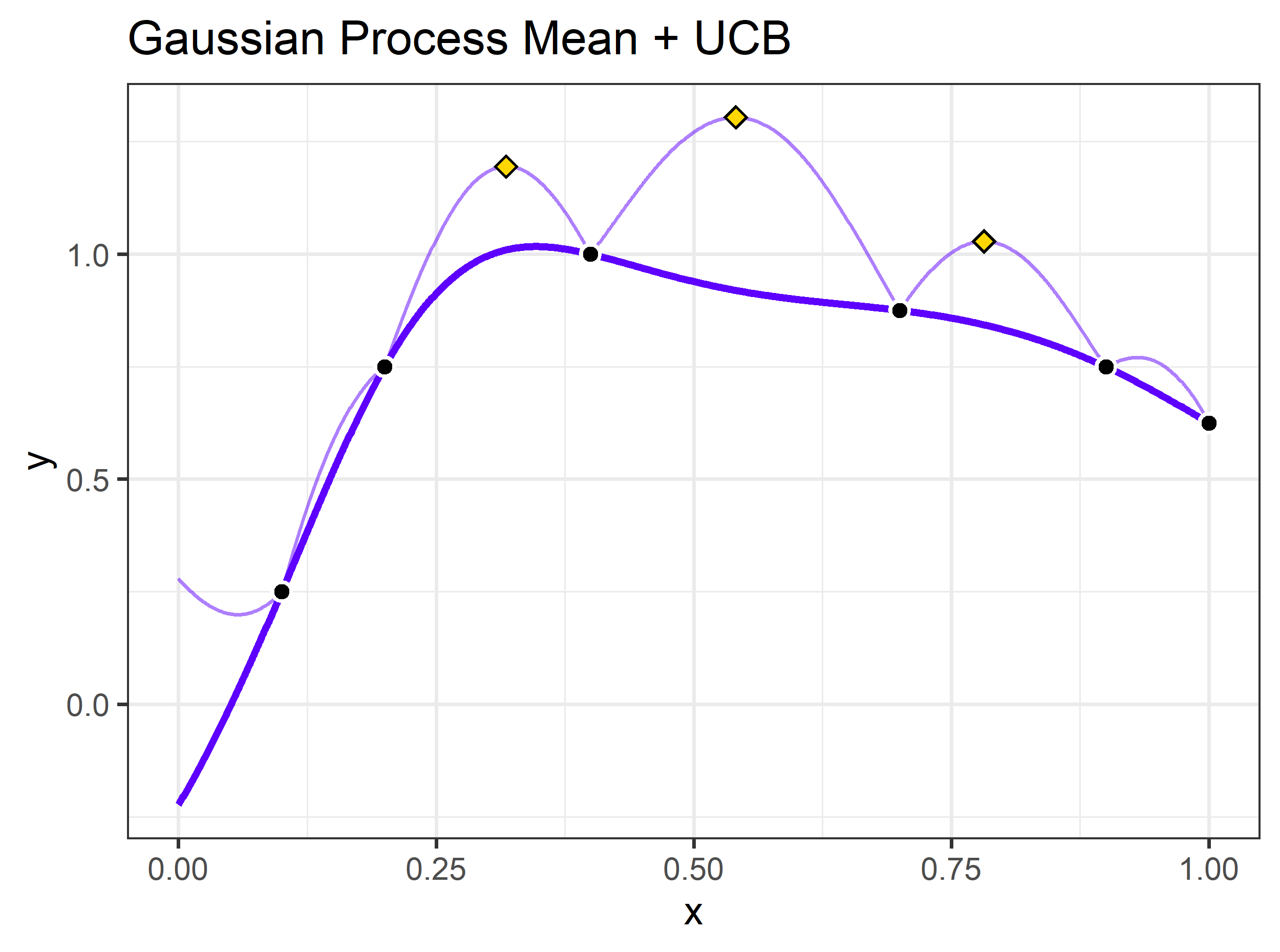
In this case, there are 3 promising candidate parameters: x ~
[0.318,0.541,0.782] with corresponding upper confidence bounds of y ~
[1.195,1.304,1.029], respectively. We may want to run our scoring
function on several of the local maximums. If acqThresh is
set to be below 1.029/1.304 ~ 0.789 and iters.k is set to
at least 3, the process would use all 3 of the local maximums as
candidate parameter sets in the next round of scoring function runs.
Going back to the example in Simple
Example, (if you let this run for a few more iterations and set
plotProgress = TRUE) you will notice this chart is updated
at each iteration:
optObjSimp <- addIterations(optObjSimp,2,verbose=FALSE)
plot(optObjSimp)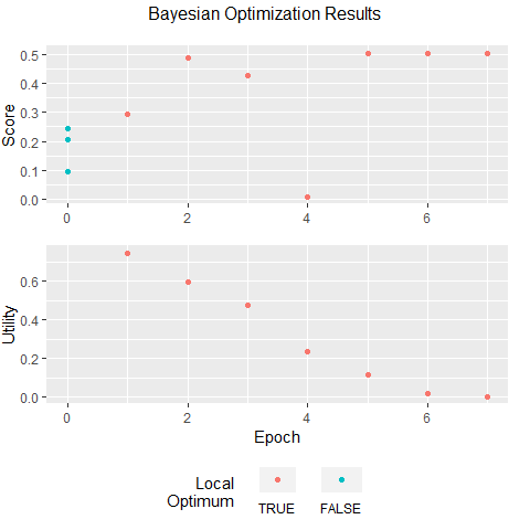
As you thoroughly explore the parameter space, you reduce the uncertainty in the unexplored areas. As you reduce uncertainty, you tend to reduce utility, which can be thought of as the potential to find a better parameter set than the one you already have. Notice that the expected improvement converged to 0 after iteration 5. If you see a similar pattern, you can be fairly certain that you have found an (approximately) global optimum.
Many times the scoring function can vary in its completion time. It
may be difficult for the user to forecast how long a single run will
take, let alone X sequential runs. For this reason, you can set a time
limit. You can also set a minimum utility limit, or you can set
both, in which case the process stops when either condition is
met. You can see how the process stopped by viewing the
stopStatus element in the returned object:
set.seed(0)

tNoPar <- system.time(
  optObj <- bayesOpt(
      FUN = scoringFunction
    , bounds = bounds
    , initPoints = 4
    , iters.n = 400
    , iters.k = 1
    , otherHalting = list(timeLimit = 5)
  )
)

optObj$stopStatus
#> [1] "Time Limit - 5 seconds."
#> attr(,"class")
#> [1] "stopEarlyMsg"
These binaries (installable software) and packages are in development.
They may not be fully stable and should be used with caution. We make no claims about them.