The hardware and bandwidth for this mirror is donated by METANET, the Webhosting and Full Service-Cloud Provider.
If you wish to report a bug, or if you are interested in having us mirror your free-software or open-source project, please feel free to contact us at mirror[@]metanet.ch.
The Ensemble Quadratic and Affine Invariant Markov chain Monte Carlo (MCMC) algorithms in the ‘QAEnsemble’ package provide an efficient way to perform Bayesian inference in difficult parameter space geometries. The Ensemble Quadratic Monte Carlo algorithm was developed by Militzer (2023) doi:10.3847/1538-4357/ace1f1. The Ensemble Affine Invariant algorithm was developed by Goodman and Weare (2010) doi:10.2140/camcos.2010.5.65 and it was implemented in Python by Foreman-Mackey, Hogg, Lang, and Goodman (2013) doi:10.48550/arXiv.1202.3665. The Quadratic Monte Carlo method was shown to perform better than the Affine Invariant method in the 2023 paper by Militzer doi:10.3847/1538-4357/ace1f1 and the Quadratic Monte Carlo method is the default method used in the Ensemble MCMC algorithm. The Chen-Shao Highest Posterior Density (HPD) Estimation algorithm is used for obtaining credible intervals and the potential scale reduction factor diagnostic is used for checking the convergence of the MCMC chains.
You can install the ‘QAEnsemble’ package from CRAN with the following command in the console:
install.packages("QAEnsemble")Ensemble Quadratic MCMC algorithm example for fitting a Weibull distribution:
library(QAEnsemble)

#Assume the true parameters are

a_shape = 20
sigma_scale = 900

#Random sample from the Weibull distribution with a = 20 and sigma = 900,
#Y~WEI(a = 20, sigma = 900)

num_ran_samples = 50

data_weibull = matrix(NA, nrow = 1, ncol = num_ran_samples)

#Set the seed for this example
set.seed(10)

data_weibull = rweibull(num_ran_samples, shape = a_shape, scale = sigma_scale)

#We want to estimate a_shape and sigma_scale

#Log prior function for a_shape and sigma_scale
#(assumed priors a_shape ~ U(1e-2, 1e2) and sigma_scale ~ U(1, 1e4))
logp <- function(param)
{
  a_shape_use = param[1]
  sigma_scale_use = param[2]

  logp_val = dunif(a_shape_use, min = 1e-2, max = 1e2, log = TRUE) +
    dunif(sigma_scale_use, min = 1, max = 1e4, log = TRUE)

  return(logp_val)
}

#Log likelihood function for a_shape and sigma_scale
logl <- function(param)
{
  a_shape_use = param[1]
  sigma_scale_use = param[2]

  logl_val = sum(dweibull(data_weibull, shape = a_shape_use, scale = sigma_scale_use, log = TRUE))

  return(logl_val)
}

logfuns = list(logp = logp, logl = logl)

num_par = 2

#It is recommended to use at least twice as many chains as the number of
#parameters to be estimated.
num_chains = 2*num_par

#Generate initial guesses for the MCMC chains
theta0 = matrix(0, nrow = num_par, ncol = num_chains)

temp_val = 0
j = 0

while(j < num_chains)
{
  initial = c(runif(1, 1e-2, 1e2), runif(1, 1, 1e4))
  temp_val = logl(initial) + logp(initial)

  while(is.na(temp_val) || is.infinite(temp_val))
  {
    initial = c(runif(1, 1e-2, 1e2), runif(1, 1, 1e4))
    temp_val = logl(initial) + logp(initial)
  }

  j = j + 1

  message(paste('j:', j))

  theta0[1,j] = initial[1]
  theta0[2,j] = initial[2]

}
#> j: 1
#> j: 2
#> j: 3
#> j: 4

num_chain_iterations = 1e4
thin_val_par = 10

#The total number of returned samples is given by
#(num_chain_iterations/thin_val_par)*num_chains = 4e3

#Ensemble Quadratic MCMC algorithm

Weibull_Quad_result = ensemblealg(theta0, logfuns, T_iter = num_chain_iterations, Thin_val = thin_val_par)

my_samples = Weibull_Quad_result$theta_sample

my_log_prior = Weibull_Quad_result$log_prior_sample

my_log_like = Weibull_Quad_result$log_like_sample

#Burn-in 25% of each chain
my_samples_burn_in = my_samples[,,-c(1:floor((num_chain_iterations/thin_val_par)*0.25))]

my_log_prior_burn_in = my_log_prior[,-c(1:floor((num_chain_iterations/thin_val_par)*0.25))]

my_log_like_burn_in = my_log_like[,-c(1:floor((num_chain_iterations/thin_val_par)*0.25))]

#Calculate potential scale reduction factors
diagnostic_result = psrfdiagnostic(my_samples_burn_in, 0.05)

diagnostic_result$p_s_r_f_vec
#>         [,1]    [,2]
#> [1,] 1.00449 1.01957

#log unnormalized posterior samples
log_un_post_vec = as.vector(my_log_prior_burn_in + my_log_like_burn_in)

#a_shape posterior samples
k1 = as.vector(my_samples_burn_in[1,,])

#sigma_scale posterior samples
k2 = as.vector(my_samples_burn_in[2,,])

#Calculate posterior median, 95% credible intervals, and maximum posterior for
#the parameters
median(k1)
#> [1] 23.93908
hpdparameter(k1, 0.05)
#> [1] 19.18364 29.35599

median(k2)
#> [1] 906.0111
hpdparameter(k2, 0.05)
#> [1] 894.9676 917.4817

k1[which.max(log_un_post_vec)]
#> [1] 24.05221

k2[which.max(log_un_post_vec)]
#> [1] 905.5819

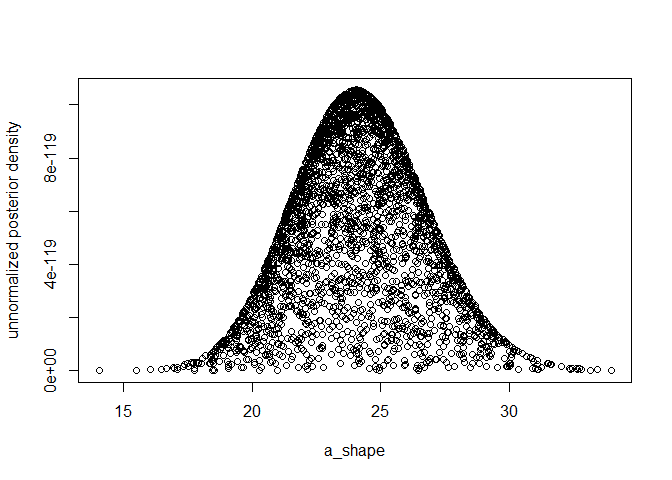
plot(k1, exp(log_un_post_vec), xlab="a_shape", ylab="unnormalized posterior density")
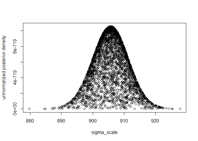
plot(k2, exp(log_un_post_vec), xlab="sigma_scale", ylab="unnormalized posterior density") ##
Progress Bar
If the ‘svMisc’ package is installed and loaded, then the progress bar in the ‘ensemblealg’ function by setting the input parameter ‘ShowProgress’ to TRUE:
ensemblealg(theta0, logfuns, T_iter = num_chain_iterations, Thin_val = thin_val_par, ShowProgress = TRUE)
If the ‘coda’ package is installed and loaded, then the ‘coda’ package ‘mcmc.list’ object is returned along with the other outputs of the ‘ensemblealg’ function by setting the input parameter ‘ReturnCODA’ to TRUE:
ensemblealg(theta0, logfuns, T_iter = num_chain_iterations, Thin_val = thin_val_par, ReturnCODA = TRUE)
Militzer B (2023) Study of Jupiter’s Interior with Quadratic Monte Carlo Simulations. ApJ 953(111):20pp. https://doi.org/10.3847/1538-4357/ace1f1
Goodman J and Weare J (2010) Ensemble samplers with affine invariance. Commun Appl Math Comput Sci 5(1):65-80. https://doi.org/10.2140/camcos.2010.5.65
Foreman-Mackey D, Hogg DW, Lang D, Goodman J (2013) emcee: The MCMC Hammer. PASP 125(925):306. https://doi.org/10.48550/arXiv.1202.3665
Chen M, Shao Q, Ibrahim JG (2000) Monte Carlo Methods in Bayesian Computation. New York-New York: Springer-Verlag.
Brooks SP and Gelman A (1998) General methods for monitoring convergence of iterative simulations. J Comp Graph Stat 7(4):434-455.
These binaries (installable software) and packages are in development.
They may not be fully stable and should be used with caution. We make no claims about them.