The hardware and bandwidth for this mirror is donated by METANET, the Webhosting and Full Service-Cloud Provider.
If you wish to report a bug, or if you are interested in having us mirror your free-software or open-source project, please feel free to contact us at mirror[@]metanet.ch.
The goal of QuantileModels is to provide the proper tools for the estimation and inference of different quantile models, at the moment only Conditional autoregressive value at risk (CAViaR) model proposed by Engle & Manganelli (2004) https://doi.org/10.1198/073500104000000370 and it’s multivariate extension MVMQ-CAViaR proposed y White et al. (2015) https://doi.org/10.1016/j.jeconom.2015.02.004 are available, however, in further updates, other models and extensions will be included.
You can install the development version of QuantileModels like so:
library(remotes)
install_github("ChJoCa/QuantileModels")
Or (only Windows users) if you don’t want, or find
difficult to install the proper tools to compile the source code, it’s
possible to download the windows binary .zip file from the
Releases section.
Here there are some examples to the estimation of the models implemented by now.
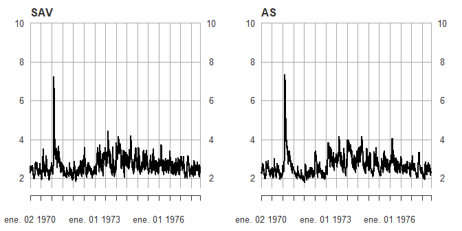
The first are the Symmetric absolute value and the Asymmetric Slope models from Engle and Manganelli (2004). Of course, there are other specifications, and all can be estimated for a given order of p autoregressive quantile and q order of lagged Y values.
library(QuantileModels)

data=dataCAViaR

SAV <- CAViaR(Y=data$GM[1:2892],
model.type = "SAV",p=1,q=1,band.hs = TRUE,quant.type = 7,
tau=0.05,refine.estim = FALSE)
#> Begining optimization
#> Calculating Standard Errors

summary(SAV)
#> CAViaR estimation
#> -------------------
#> Model specification: SAV
#> Quantile (tau): 0.05
#> Loss function value at estimates: 551.2903
#> In-sample coverage: 0.05014
#> Hall-Sheather bandwidth
#>
#> Estimation results:
#> ========================================================
#>            Coef.     S.E   P>|t|  2.5% CI 97.5% CI
#> Beta 0  -0.15817 0.09835 0.10788 -0.35102  0.03467
#> Beta 1   0.88566 0.04309 0.00000  0.80118  0.97014
#> Gamma 1 -0.11445 0.01711 0.00000 -0.14800 -0.08091
#> ========================================================
#>
#> Coverage test
#> -------------------
#> Kupiec conditional coverage test (LRcc), p-value: 0.91283
#> Christoffersen independence test (LRind), p-value: 0.67031
#> Christoffersen unconditional coverage test (LRuc), p-value: 0.97279

AS <- CAViaR(Y=data$GM[1:2892],
model.type = "AS",p=1,q=1,band.hs = TRUE,quant.type = 7,
tau=0.05,refine.estim = FALSE)
#> Begining optimization
#> Calculating Standard Errors

summary(AS)
#> CAViaR estimation
#> -------------------
#> Model specification: AS
#> Quantile (tau): 0.05
#> Loss function value at estimates: 548.3021
#> In-sample coverage: 0.04945
#> Hall-Sheather bandwidth
#>
#> Estimation results:
#> ========================================================
#>             Coef.     S.E   P>|t|  2.5% CI 97.5% CI
#> Beta 0   -0.07599 0.03250 0.01944 -0.13971 -0.01227
#> Beta 1    0.93262 0.01424 0.00000  0.90470  0.96054
#> Gamma+,1 -0.03977 0.02103 0.05876 -0.08101  0.00147
#> Gamma-,1  0.12179 0.01453 0.00000  0.09330  0.15027
#> ========================================================
#>
#> Coverage test
#> -------------------
#> Kupiec conditional coverage test (LRcc), p-value: 0.64971
#> Christoffersen independence test (LRind), p-value: 0.35833
#> Christoffersen unconditional coverage test (LRuc), p-value: 0.89123
graphic_opts <- par(no.readonly = TRUE)
par(mfrow=c(1,2))

plot(-SAV$VaR,.by="quarter",ylim=c(1.5,10),main="SAV",main.timespan=FALSE)
plot(-AS$VaR,.by="quarter",ylim=c(1.5,10),main="AS",main.timespan=FALSE)
par(graphic_opts)The other model is it’s multivariate version proposed by White et al. (2015)
Barclays <- MVMQ_CAViaR(MVMQ[,c(6,1)],tau =c(0.01,0.01),band.hs = TRUE)
#> Begining optimization
#> Calculating Standard Errors

summary(Barclays)
#> MVMQ CAViaR estimation
#> Loss function at estimates: 324.0218
#> Hall-Sheather bandwidth
#> ========================================================
#> Equation: yEU_index
#> Quantile (tau): 0.01
#> In sample coverage 0.01049
#> Estimation results:
#> --------------------------------------------------------
#>                               Coef.     S.E   P>|t|  2.5% CI 97.5% CI
#> Const.                     -0.13209 0.04568 0.00387 -0.22166 -0.04251
#> q.yEU_index,1               0.80808 0.04854 0.00000  0.71290  0.90326
#> q.BARCLAYS - PRICE INDEX,1 -0.01093 0.00695 0.11565 -0.02455  0.00269
#> |yEU_index|,1              -0.51111 0.12095 0.00002 -0.74827 -0.27395
#> |BARCLAYS - PRICE INDEX|,1 -0.05018 0.01083 0.00000 -0.07142 -0.02894
#>
#> Coverage test
#> -------------------
#> Kupiec conditional coverage test (LRcc), p-value: 0.70412
#> Christoffersen independence test (LRind), p-value: 0.42513
#> Christoffersen unconditional coverage test (LRuc), p-value: 0.79796
#> --------------------------------------------------------
#>
#> Equation: BARCLAYS - PRICE INDEX
#> Quantile (tau): 0.01
#> In sample coverage 0.00976
#> Estimation results:
#> --------------------------------------------------------
#>                               Coef.     S.E   P>|t|  2.5% CI 97.5% CI
#> Const.                     -0.09075 0.04920 0.06519 -0.18722  0.00571
#> q.yEU_index,1              -0.12595 0.06035 0.03697 -0.24428 -0.00762
#> q.BARCLAYS - PRICE INDEX,1  0.95959 0.01066 0.00000  0.93868  0.98049
#> |yEU_index|,1              -0.33446 0.12710 0.00855 -0.58369 -0.08524
#> |BARCLAYS - PRICE INDEX|,1 -0.14545 0.07610 0.05608 -0.29467  0.00378
#>
#> Coverage test
#> -------------------
#> Kupiec conditional coverage test (LRcc), p-value: 0.08638
#> Christoffersen independence test (LRind), p-value: 0.02713
#> Christoffersen unconditional coverage test (LRuc), p-value: 0.90074
#> --------------------------------------------------------

dates <- as.Date(zoo::index(MVMQ))

plot(dates,as.vector(MVMQ[,1]),type = "p",ylim = c(-60,60),cex=0.6,xaxt="n",cex.axis=0.8,col=2,xlab="",ylab = "",main = "Barclays")
lines(dates,Barclays[[5]][,2],type = "l")
axis.Date(side=1,at=seq(dates[1],dates[2765],by="year"),cex.axis=0.8,las=2)
legend("topleft",legend = c("Daily Returns","1% VaR"),col = 2:1,pch = c("o","-"))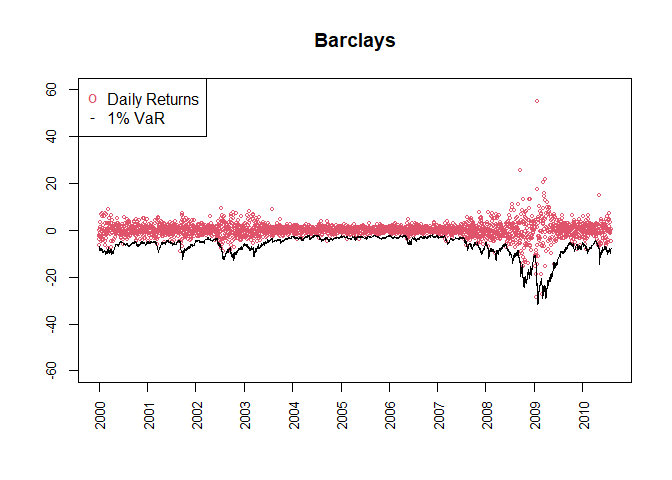
These binaries (installable software) and packages are in development.
They may not be fully stable and should be used with caution. We make no claims about them.