The hardware and bandwidth for this mirror is donated by METANET, the Webhosting and Full Service-Cloud Provider.
If you wish to report a bug, or if you are interested in having us mirror your free-software or open-source project, please feel free to contact us at mirror[@]metanet.ch.

RBaM - An R user interface to BaM

Introduction

BaM (Bayesian Modeling) is a framework to estimate a model using Bayesian inference. The R package RBaM is built as an R User Interface to the computational BaM engine. It defines classes (objects’ properties and methods) for the various building blocks of a BaM case study. Its typical usage is as follows:

Assemble the dataset of input/ouput variables.
Define the model and set prior distributions for its parameters.
Perform Bayesian-MCMC inference.
Perform predictions.

# devtools::install_github('BaM-tools/RBaM') # First use: install the package from GitHub
library(RBaM) # Load package

The catalogue of distributions and models that are available in RBaM can be accessed as follows:

getCatalogue()

## $distributions
##  [1] "Gaussian"     "Uniform"      "Triangle"     "LogNormal"    "LogNormal3"  
##  [6] "Exponential"  "GPD"          "Gumbel"       "GEV"          "GEV_min"     
## [11] "Inverse_Chi2" "PearsonIII"   "Geometric"    "Poisson"      "Bernoulli"   
## [16] "Binomial"     "NegBinomial"  "FlatPrior"    "FlatPrior+"   "FlatPrior-"  
## [21] "FIX"          "VAR"         
## 
## $models
##  [1] "TextFile"                 "BaRatin"                 
##  [3] "BaRatinBAC"               "SFD"                     
##  [5] "SGD"                      "SWOT"                    
##  [7] "Vegetation"               "AlgaeBiomass"            
##  [9] "DynamicVegetation"        "Recession_h"             
## [11] "Segmentation"             "Sediment"                
## [13] "SuspendedLoad"            "Linear"                  
## [15] "Mixture"                  "Orthorectification"      
## [17] "GR4J"                     "Tidal"                   
## [19] "SFDTidal"                 "SFDTidal2"               
## [21] "SFDTidalJones"            "SFDTidal4"               
## [23] "SFDTidal_Qmec0"           "SFDTidal_Qmec"           
## [25] "SFDTidal_Qmec2"           "TidalODE"                
## [27] "TidalRemenieras"          "SFDTidal_Sw_correction"  
## [29] "MAGE"                     "MAGE_TEMP"               
## [31] "HydraulicControl_section"

An example using the BaRatin rating curve model

A rating curve is a model linking the water stage \(H\) measured at a given point of a river and the discharge \(Q\) flowing through it. The elementary rating curve equation has the power-law form Q=a(H-b)^c, where a, b and c are parameters. Since different hydraulic controls may succeed to each other as the water stage increases, it is frequent to use a piecewise combination of these elementary equations, for instance: Q=a₁(H-b₁)^c₁ for k₁ < H < k₂; Q=a₂(H-b₂)^c₂ for H > k₂, with k₁ and k₂ the activation stages of the first and the second control. We refer to this article for additional details.

This example shows how to estimate a rating curve using a set of (H,Q) calibration data (called ‘gaugings’) from the Ardèche river at the Sauze-Saint-Martin hydrometric station. The first thing to do is to define the workspace, i.e. the folder where configuration and result files will be written.

workspace=file.path(tempdir(),'BaM_workspace')

The second step is to define the calibration data. The dataset SauzeGaugings is provided with this package, and the code below let RBaM know what to use as inputs/outputs.

# Define the calibration dataset by specifying 
# inputs (X), outputs (Y) and uncertainty on the outputs (Yu).
# A copy of this dataset will be written in data.dir.
D=dataset(X=SauzeGaugings['H'],Y=SauzeGaugings['Q'],Yu=SauzeGaugings['uQ'],data.dir=workspace)

The third step is to define the rating curve model. The code below specifies the priors on parameters, the control matrix and creates the model object.

# Parameters of the low flow section control: activation stage k, coefficient a and exponent c
k1=parameter(name='k1',init=-0.5,prior.dist='Uniform',prior.par=c(-1.5,0))
a1=parameter(name='a1',init=50,prior.dist='LogNormal',prior.par=c(log(50),1))
c1=parameter(name='c1',init=1.5,prior.dist='Gaussian',prior.par=c(1.5,0.05))
# Parameters of the high flow channel control: activation stage k, coefficient a and exponent c
k2=parameter(name='k2',init=1,prior.dist='Gaussian',prior.par=c(1,1))
a2=parameter(name='a2',init=100,prior.dist='LogNormal',prior.par=c(log(100),1))
c2=parameter(name='c2',init=1.67,prior.dist='Gaussian',prior.par=c(1.67,0.05))
# Define control matrix: columns are controls, rows are stage ranges.
# Here the matrix means that the first control only is active for the first stage range,
# and the second control only is active for the second stage range.
controlMatrix=rbind(c(1,0),c(0,1))
# Stitch it all together into a model object
M=model(ID='BaRatin',
        nX=1,nY=1, # number of input/output variables
        par=list(k1,a1,c1,k2,a2,c2), # list of model parameters
        xtra=xtraModelInfo(object=controlMatrix)) # use xtraModelInfo() to pass the control matrix

All set! The function BaM can now be called to estimate parameters. This will run a MCMC sampler and save the result into the workspace.

BaM(workspace=workspace,mod=M,data=D)

MCMC samples can now be read. There are 2 MCMC files: ‘Results_MCMC.txt’ contains raw MCMC simulations and is hence quite big. ‘Results_Cooking.txt’ contains ‘cooked’ simulations, i.e. after ‘burning’ the first part of iterations and ‘slicing’ what remains, and may be favored in most cases. Functions mcmcOptions and mcmcCooking allow controlling MCMC properties.

# Read 'cooked' MCMC file in the workspace
MCMC=readMCMC(file.path(workspace,'Results_Cooking.txt'))
head(MCMC)

##          k1      a1      c1       k2       a2      c2    Y1_g1     Y1_g2
## 1 -0.246780 60.4238 1.48103 0.922899 102.8730 1.70117 2.582080 0.0224468
## 2 -0.269413 60.5724 1.46413 0.930665  99.0574 1.70117 2.232150 0.0131388
## 3 -0.291071 58.2851 1.51878 1.000870 105.3410 1.71316 1.904870 0.0157354
## 4 -0.327582 55.5986 1.50333 1.053400 108.8020 1.67034 2.385710 0.0118051
## 5 -0.346240 53.3239 1.50333 1.087950 120.9590 1.66413 0.756269 0.0414687
## 6 -0.353747 51.7361 1.49109 1.045050 110.3710 1.69349 0.590987 0.0467566
##    LogPost        b1        b2
## 1 -153.555 -0.246780 0.0845701
## 2 -152.904 -0.269413 0.0544618
## 3 -151.209 -0.291071 0.1125240
## 4 -150.324 -0.327582 0.1588370
## 5 -146.927 -0.346240 0.2412690
## 6 -145.997 -0.353747 0.1859880

A few functions are provided with the package to explore MCMC samples.

# Trace plot for each parameter, useful to assess convergence.
plots=tracePlot(MCMC)
gridExtra::grid.arrange(grobs=plots,ncol=3)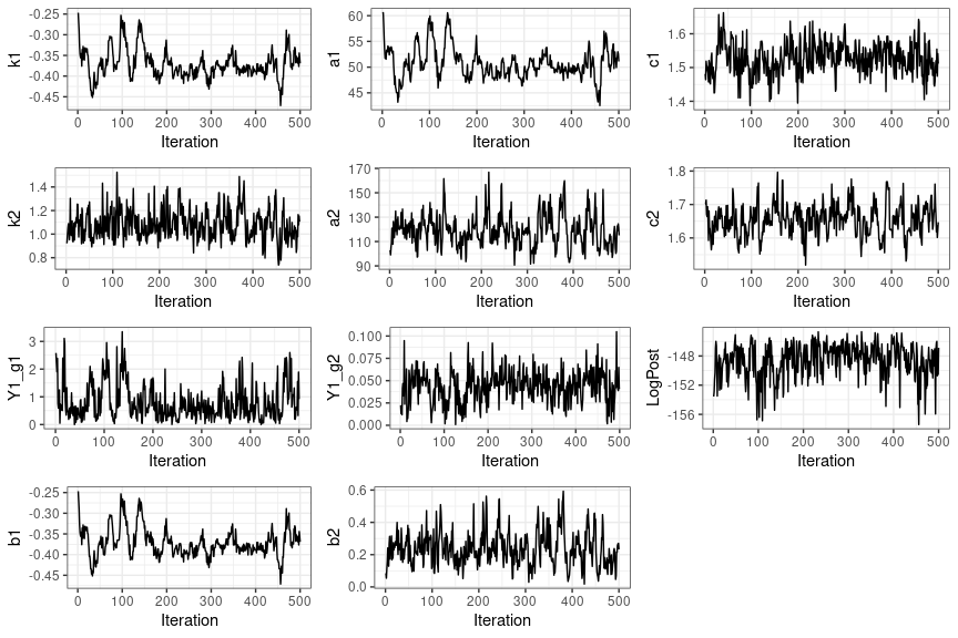

# Density plot for each parameter
plots=densityPlot(MCMC)
gridExtra::grid.arrange(grobs=plots,ncol=3)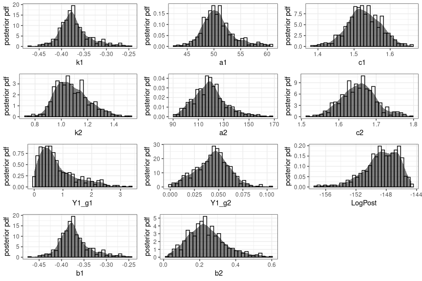

# Violon plot, useful to compare 'comparable' parameters.
violinPlot(MCMC[c('c1','c2')])

Finally, the estimated rating curve model can be used to make predictions as shown below.

# Define the grid of stage values on which the rating curve will be computed
hgrid=data.frame(H=seq(-1,7,0.1))
# Define a 'prediction' object for total predictive uncertainty
totalU=prediction(X=hgrid, # stage values
                  spagFiles='totalU.spag', # file where predictions are saved
                  data.dir=workspace, # a copy of data files will be saved here
                  doParametric=TRUE, # propagate parametric uncertainty, i.e. MCMC samples?
                  doStructural=TRUE) # propagate structural uncertainty ?
# Define a 'prediction' object for parametric uncertainty only - not the doStructural=FALSE
paramU=prediction(X=hgrid,spagFiles='paramU.spag',data.dir=workspace,
                  doParametric=TRUE,doStructural=FALSE)
# Define a 'prediction' object with no uncertainty - this corresponds to the 'maxpost' rating curve maximizing the posterior
maxpost=prediction(X=hgrid,spagFiles='maxpost.spag',data.dir=workspace,
                  doParametric=FALSE,doStructural=FALSE)
# Re-run BaM, but in prediction mode
BaM(workspace=workspace,mod=M,data=D, # model and data
    pred=list(totalU,paramU,maxpost), # list of predictions
    doCalib=FALSE,doPred=TRUE) # Do not re-calibrate but do predictions

The resulting ‘spaghetti files’ can be read into the workspace and plotted.

# Plot spaghetti representing total uncertainty in red
Q=read.table(file.path(workspace,'totalU.spag'))
matplot(hgrid$H,Q,col='red',type='l',lty=1)
# Add spaghetti representing parametric uncertainty in pink
Q=read.table(file.path(workspace,'paramU.spag'))
matplot(hgrid$H,Q,col='pink',type='l',lty=1,add=TRUE)
# Add maxpost rating curve
Q=read.table(file.path(workspace,'maxpost.spag'))
matplot(hgrid$H,Q,col='black',type='l',lty=1,add=TRUE)

Spaghetti are the raw outputs of the predictions, but it is often more convenient to plot probability intervals only. These have been computed automatically by BaM, and are saved in files with an ‘.env’ (like ‘envelop’) extension.

Q=read.table(file.path(workspace,'totalU.env'),header=T)
matplot(hgrid$H,Q[,2:3],col='red',type='l',lty=1)
Q=read.table(file.path(workspace,'paramU.env'),header=T)
matplot(hgrid$H,Q[,2:3],col='pink',type='l',lty=1,add=TRUE)
Q=read.table(file.path(workspace,'maxpost.spag'))
matplot(hgrid$H,Q,col='black',type='l',lty=1,add=TRUE)

These binaries (installable software) and packages are in development.
They may not be fully stable and should be used with caution. We make no claims about them.