The hardware and bandwidth for this mirror is donated by METANET, the Webhosting and Full Service-Cloud Provider.
If you wish to report a bug, or if you are interested in having us mirror your free-software or open-source project, please feel free to contact us at mirror[@]metanet.ch.
The goal of SSOSVM is to use R to allow batch and online training of soft-margin support vector machines (SVMs). The training of SVMs usually requires that the data be available all at once in a single batch, however the Stochastic majorization-minimization (SMM) algorithm framework allows for the training of SVMs on streamed data instead http://doi.org/10.1007/s42081-018-0001-y. This package utilizes the SMM framework to provide functions for training SVMs with hinge loss, squared-hinge loss, and logistic loss, functions.
You can install SSOSVM from github with:
# install.packages("devtools")
devtools::install_github("andrewthomasjones/SSOSVM")Here is a very simple example using simulated data:
#setup
library(SSOSVM)
library(ggplot2)
#> Warning: package 'ggplot2' was built under R version 4.4.1

#simulations
sims <- generateSim(100, DELTA=3)

#fit using various loss functions
sq1<-SVMFit(sims$YMAT,"square")
h1<-SVMFit(sims$YMAT,"hinge")
l1<-SVMFit(sims$YMAT,"logistic")

#plot results
plot<-ggplot(data.frame(sims$YMAT), aes(colour=factor(YY), x=V2, y=V3))
plot<-plot+geom_point()+theme_bw()+xlab("X")+ylab("Y")+guides(colour=FALSE)
#> Warning: The `<scale>` argument of `guides()` cannot be `FALSE`. Use "none" instead as
#> of ggplot2 3.3.4.
#> This warning is displayed once every 8 hours.
#> Call `lifecycle::last_lifecycle_warnings()` to see where this warning was
#> generated.
plot<-plot+geom_abline(intercept=sq1$THETA[1],
                       slope=sq1$THETA[2]/sq1$THETA[3], colour="blue")
plot<-plot+geom_abline(intercept=h1$THETA[1],
                       slope=h1$THETA[2]/h1$THETA[3], colour="green")
plot<-plot+geom_abline(intercept=l1$THETA[1],
                       slope=l1$THETA[2]/l1$THETA[3], colour="red")
plot
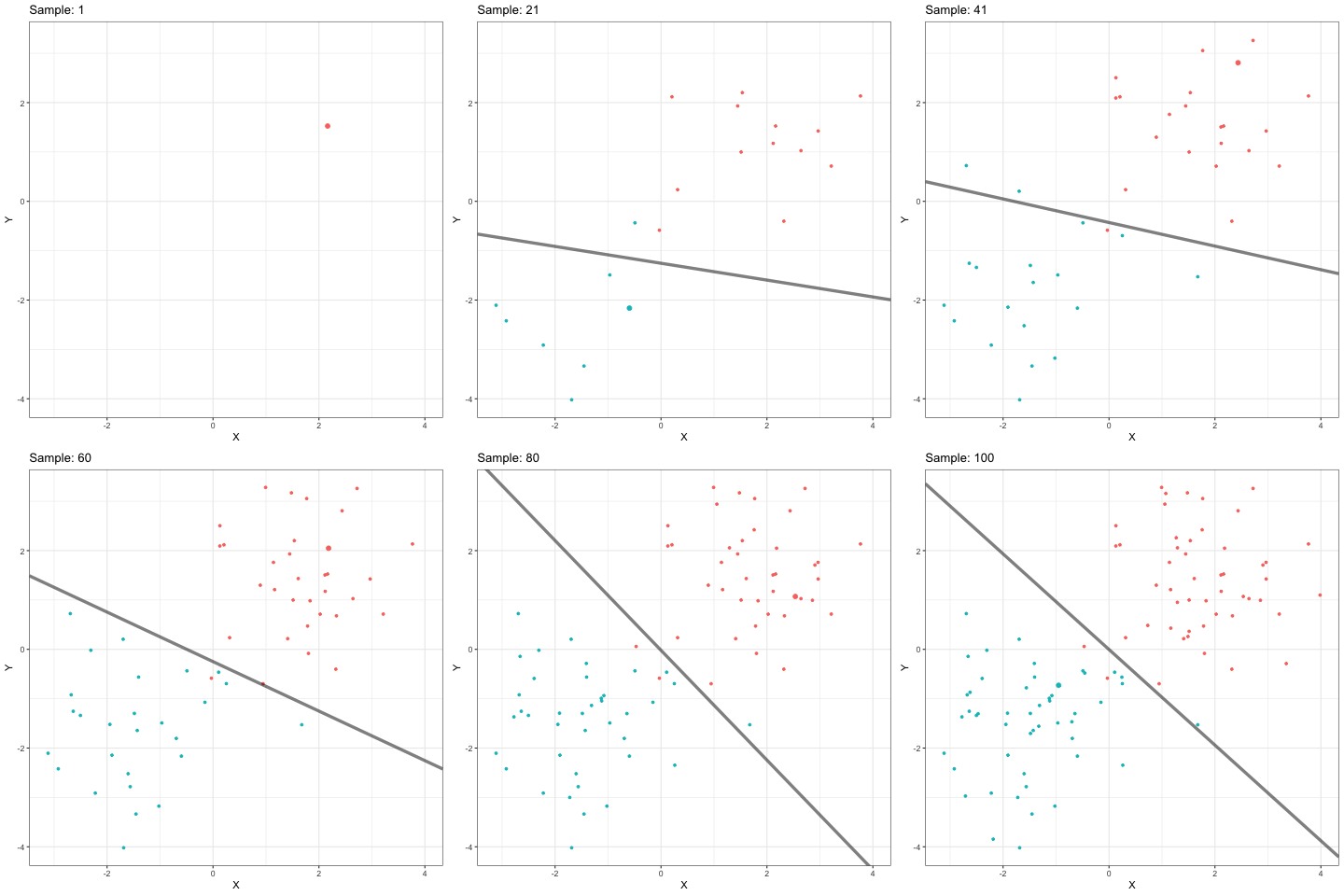
Here is an animated example to demostrate the online nature of of the SSOSVM method:
library(ggplot2)
library(gganimate)

#set up
sims <- generateSim(10^2, DELTA=1.5)

#fit using various loss functions
sq1<-SVMFit(sims$YMAT,"square", returnAll = TRUE)
h1<-SVMFit(sims$YMAT,"hinge", returnAll = TRUE)
l1<-SVMFit(sims$YMAT,"logistic", returnAll = TRUE)

#dataframe
data<-data.frame(sample=1:10^2,
                 sims$YMAT,
                 logistic_int=l1$THETA_list[,1],
                 square_int=sq1$THETA_list[,1],
                 hinge_int=h1$THETA_list[,1],
                 logistic_sl=l1$THETA_list[,2]/l1$THETA_list[,3],
                 square_sl=sq1$THETA_list[,2]/sq1$THETA_list[,3],
                 hinge_sl=h1$THETA_list[,2]/h1$THETA_list[,3])

#base plot
plot<-ggplot(data, aes(colour=factor(YY), x=V2, y=V3))+
  geom_point(size=2)+theme_bw()+xlab("X")+ylab("Y")+
  guides(colour=FALSE)+geom_abline(size=1.6,alpha=.5, aes(intercept=square_int, slope=square_sl))

#animate
example <- plot + transition_time(sample)+
  labs(title =  "Sample: {frame_time}")+
  shadow_mark(alpha = 1, size = 1, exclude_layer = 2)

#save animation
anim_save("./inst/example.gif", example, fps=2.5)
These binaries (installable software) and packages are in development.
They may not be fully stable and should be used with caution. We make no claims about them.