The hardware and bandwidth for this mirror is donated by METANET, the Webhosting and Full Service-Cloud Provider.
If you wish to report a bug, or if you are interested in having us mirror your free-software or open-source project, please feel free to contact us at mirror[@]metanet.ch.
![]()
![]()
With the growth of big data, variable selection has become one of the major challenges in statistics. Although many methods have been proposed in the literature their performance in terms of recall and precision are limited in a context where the number of variables by far exceeds the number of observations or in a high correlated setting.
SelectBoost.beta brings the correlation-aware resampling
strategy of the original SelectBoost package to beta
regression by implementing an extension of the
SelectBoost algorithm, F. Bertrand, I. Aouadi, N. Jung,
R. Carapito, L. Vallat, S. Bahram, M. Maumy-Bertrand (2015) https://doi.org/10.1093/bioinformatics/btaa855 and https://doi.org/10.32614/CRAN.package.SelectBoost.
It ships with:
betareg_step_aic() and
betareg_glmnet() that act as base selectors for
beta-distributed outcomes, now including optional precision (phi)
submodel search and observation weights;sb_normalize(),
sb_group_variables(), sb_resample_groups(), …)
mirroring the core stages of SelectBoost; andsb_beta() driver that orchestrates
normalisation, correlation analysis, grouped resampling and stability
tallying in a single call.SelectBoost.beta ships with multiple selector families.
Use the table below as a starting point when deciding which helper best
matches your workflow:
| Selector | What it does | Good defaults for | Extra packages |
|---|---|---|---|
betareg_step_aic() / betareg_step_bic() /
betareg_step_aicc() |
Greedy stepwise search on betareg fits (mean submodel,
optional phi search) using the chosen information criterion. |
Small-to-moderate p, interpretable models, when you
want to reuse betareg summaries. |
betareg (installed automatically). |
betareg_glmnet() |
Iteratively reweighted least squares with glmnet on the
working responses; supports AIC/BIC/CV selection. |
Higher-dimensional settings or when you need elastic-net regularisation with no extra dependencies. | glmnet. |
betareg_lasso_gamlss() |
LASSO penalty through gamlss::ri() on the beta mean
submodel. |
Workflows already using gamlss, or when you need
GAIC-tuned shrinkage. |
gamlss, gamlss.dist. |
betareg_enet_gamlss() |
Elastic-net variant via gamlss.lasso::gnet(). |
When elastic-net is needed alongside GAMLSS diagnostics. | gamlss, gamlss.dist,
gamlss.lasso. |
All selectors expect complete cases for the supplied design matrix and only act on the mean submodel. Offsets and observation-level weights beyond what is exposed in each helper are currently unsupported.
Each resampling call returns per-group diagnostics (cached draws,
observed correlation summaries) and sb_beta() threads the
same correlated surrogates across all thresholds so cross-level
comparisons remain aligned. Interval responses are supported through the
interval argument, which reuses the
fastboost_interval() logic directly inside
sb_beta().
The package is designed so that each stage of the workflow remains reusable on its own. Users can plug in custom grouping strategies or selectors while still benefiting from correlated resampling.
The SelectBoost4Beta approach was presented by Frédéric Bertrand and Myriam Maumy at the Joint Statistical Meetings 2023 in Toronto (“Improving variable selection in Beta regression models using correlated resampling”) and at BioC2023 in Boston (“SelectBoost4Beta: Improving variable selection in Beta regression models”). Both communications highlighted how correlated resampling boosts variable selection for Beta regression in high-dimensional, strongly correlated settings.
SelectBoost.beta is preparing for its first CRAN submission. Until it becomes available there, install the development version from GitHub:
devtools::install_github("fbertran/SelectBoost.beta")Once the package lands on CRAN, the usual
install.packages("SelectBoost.beta") command will work as
expected.
The selectors rely on the betareg, glmnet,
and gamlss ecosystems. These packages will be pulled in
automatically when installing from source.
Simulate a correlated design, run the manual SelectBoost steps with
betareg_step_aic(), and compute selection frequencies:
library(SelectBoost.beta)
set.seed(42)

sim <- simulation_DATA.beta(n = 150, p = 6, s = 3, beta_size = c(1, -0.8, 0.6))
X_norm <- sb_normalize(sim$X)
corr_mat <- sb_compute_corr(X_norm)
groups <- sb_group_variables(corr_mat, c0 = 0.6)
resamples <- sb_resample_groups(X_norm, groups, B = 50)
#> Warning: All groups are singletons; correlated resampling degenerates to repeated `X_norm`.
coef_path <- sb_apply_selector_manual(X_norm, resamples, sim$Y, betareg_step_aic)
sel_freq <- sb_selection_frequency(coef_path, version = "glmnet")
sel_freq
#>              x1              x2              x3              x4              x5              x6
#>               1               1               1               0               0               0
#> phi|(Intercept)
#>               1

attr(resamples, "diagnostics")
#>   group size regenerated cached mean_abs_corr_orig mean_abs_corr_surrogate mean_abs_corr_cross
#> 1    x1    1           0  FALSE                 NA                      NA                  NA
#> 2    x2    1           0  FALSE                 NA                      NA                  NA
#> 3    x3    1           0  FALSE                 NA                      NA                  NA
#> 4    x4    1           0  FALSE                 NA                      NA                  NA
#> 5    x5    1           0  FALSE                 NA                      NA                  NA
#> 6    x6    1           0  FALSE                 NA                      NA                  NA
The sb_beta() wrapper performs the entire loop
internally and returns a matrix indexed by the correlation thresholds
used during resampling:
sb <- sb_beta(sim$X, sim$Y, B = 50, step.num = 0.25,use.parallel = FALSE)
print(sb)
#> SelectBoost beta selection frequencies
#> Selector: betareg_step_aic
#> Resamples per threshold: 50
#> Interval mode: none
#> c0 grid: 1.000, 0.089, 0.059, 0.030, 0.000
#> Inner thresholds: 0.089, 0.059, 0.030
#>              x1   x2   x3   x4   x5   x6 phi|(Intercept)
#> c0 = 1.000 1.00 1.00 1.00 0.00 0.00 0.00               1
#> c0 = 0.089 0.24 0.14 0.14 0.18 0.14 0.18               1
#> c0 = 0.059 0.16 0.14 0.26 0.10 0.12 0.16               1
#> c0 = 0.030 0.20 0.14 0.14 0.12 0.18 0.20               1
#> c0 = 0.000 0.16 0.12 0.12 0.14 0.18 0.14               1
#> attr(,"c0.seq")
#> [1] 1.00000000 0.08894615 0.05949716 0.03010630 0.00000000
#> attr(,"steps.seq")
#> [1] 0.08894615 0.05949716 0.03010630
#> attr(,"B")
#> [1] 50
#> attr(,"selector")
#> [1] "betareg_step_aic"
#> attr(,"resample_diagnostics")
#> attr(,"resample_diagnostics")$`c0 = 1.000`
#> [1] group                   size                    regenerated             cached
#> [5] mean_abs_corr_orig      mean_abs_corr_surrogate mean_abs_corr_cross
#> <0 rows> (or 0-length row.names)
#>
#> attr(,"resample_diagnostics")$`c0 = 0.089`
#>      group size regenerated cached mean_abs_corr_orig mean_abs_corr_surrogate mean_abs_corr_cross
#> 1    x1,x4    2          50  FALSE         0.08894615              0.10146558          0.07089570
#> 2 x2,x3,x6    3          50  FALSE         0.07694401              0.09829963          0.06673431
#> 3 x2,x3,x5    3          50  FALSE         0.08217406              0.09634851          0.06390166
#> 4    x3,x5    2          50  FALSE         0.09286939              0.09536360          0.05329723
#> 5    x2,x6    2          50  FALSE         0.10556609              0.11060608          0.07179976
#>
#> attr(,"resample_diagnostics")$`c0 = 0.059`
#>            group size regenerated cached mean_abs_corr_orig mean_abs_corr_surrogate mean_abs_corr_cross
#> 1    x1,x2,x3,x4    4          50  FALSE         0.06136428              0.08621443          0.06598362
#> 2 x1,x2,x3,x5,x6    5          50  FALSE         0.06152013              0.08582089          0.06337853
#> 3    x1,x2,x3,x5    4          50  FALSE         0.07198271              0.08974742          0.06489135
#> 4       x1,x4,x5    3          50  FALSE         0.06290784              0.07535777          0.06047434
#> 5    x2,x3,x4,x5    4          50  FALSE         0.05766823              0.08028623          0.06062214
#> 6          x2,x6    2           0   TRUE         0.10556609              0.11060608          0.07179976
#>
#> attr(,"resample_diagnostics")$`c0 = 0.030`
#>               group size regenerated cached mean_abs_corr_orig mean_abs_corr_surrogate mean_abs_corr_cross
#> 1    x1,x2,x3,x4,x5    5          50  FALSE         0.06203296              0.08360476          0.06487303
#> 2    x1,x2,x3,x5,x6    5           0   TRUE         0.06152013              0.08582089          0.06337853
#> 3       x1,x4,x5,x6    4          50  FALSE         0.04694388              0.07252823          0.06954473
#> 4 x1,x2,x3,x4,x5,x6    6          50  FALSE         0.05666305              0.08518211          0.06383341
#> 5    x2,x3,x4,x5,x6    5          50  FALSE         0.05591031              0.08187888          0.06182501
#>
#> attr(,"resample_diagnostics")$`c0 = 0.000`
#>               group size regenerated cached mean_abs_corr_orig mean_abs_corr_surrogate mean_abs_corr_cross
#> 1 x1,x2,x3,x4,x5,x6    6           0   TRUE         0.05666305              0.08518211          0.06383341
#>
#> attr(,"interval")
#> [1] "none"
The result stores the selector used, the number of resamples, and the correlation thresholds in its attributes. Dedicated methods make these easier to inspect programmatically:
summary(sb)
#> SelectBoost beta summary
#> Selector: betareg_step_aic
#> Resamples per threshold: 50
#> Interval mode: none
#> c0 grid: 1.000, 0.089, 0.059, 0.030, 0.000
#> Inner thresholds: 0.089, 0.059, 0.030
#> Top rows:
#>        c0        variable frequency
#> 1  1.0000              x1      1.00
#> 2  1.0000              x2      0.24
#> 3  1.0000              x3      0.16
#> 4  1.0000              x4      0.20
#> 5  1.0000              x5      0.16
#> 6  1.0000              x6      1.00
#> 7  1.0000 phi|(Intercept)      0.14
#> 8  0.0889              x1      0.14
#> 9  0.0889              x2      0.14
#> 10 0.0889              x3      0.12
if (requireNamespace("ggplot2", quietly = TRUE)) {
  autoplot.sb_beta(sb)
}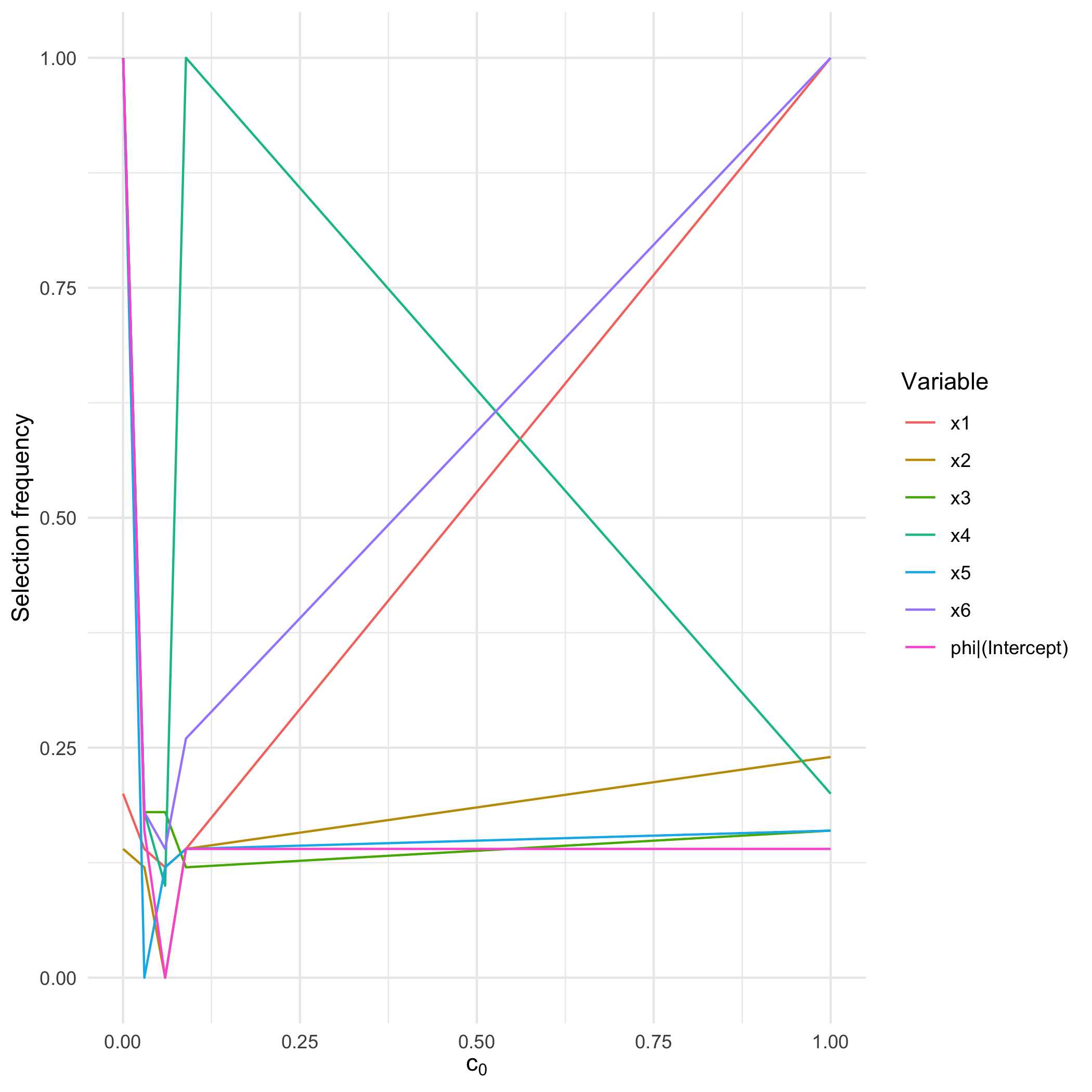
plot of chunk unnamed-chunk-4
attr(sb, "selector")
#> [1] "betareg_step_aic"
attr(sb, "c0.seq")
#> [1] 1.00000000 0.08894615 0.05949716 0.03010630 0.00000000
attr(sb, "resample_diagnostics")[[1]]
#> [1] group                   size                    regenerated             cached
#> [5] mean_abs_corr_orig      mean_abs_corr_surrogate mean_abs_corr_cross
#> <0 rows> (or 0-length row.names)sb_beta() outputThe matrix returned by sb_beta() carries a number of
attributes so downstream code can recover how the stability frequencies
were produced:
attr(sb, "c0.seq") lists the absolute-correlation
thresholds explored.attr(sb, "steps.seq") reports the raw sequence used to
build that grid when step.num was provided.attr(sb, "B") records the number of correlated
resamples per threshold.attr(sb, "selector") stores the selector name or
expression.attr(sb, "interval") highlights whether interval
resampling was used.attr(sb, "resample_diagnostics") holds per-threshold
summaries of the cached surrogate draws.These attributes mirror the original SelectBoost design and are
documented in ?sb_beta to ease CRAN review.
single <- compare_selectors_single(sim$X, sim$Y, include_enet = TRUE)compare_selectors_single() temporarily shortens column
names so that the selectors receive syntactically valid identifiers; the
returned list remaps the coefficients and long table back to the
original labels.
freq <- suppressWarnings(compare_selectors_bootstrap(
  sim$X, sim$Y, B = 100, include_enet = TRUE, seed = 321
))
head(freq)
#>    selector variable freq n_success n_fail
#> x1      AIC       x1 1.00       100      0
#> x2      AIC       x2 1.00       100      0
#> x3      AIC       x3 1.00       100      0
#> x4      AIC       x4 0.27       100      0
#> x5      AIC       x5 0.14       100      0
#> x6      AIC       x6 0.19       100      0
The freq column reports how often each variable was
selected across the bootstrap replicates, and the accompanying
n_success/n_fail counts indicate how many
resamples contributed to each estimate. Values close to 1 indicate
highly stable discoveries, whereas small values suggest weak or noisy
support. Inspect attr(freq, "failures") to review any
selector errors. Increase B when you need finer resolution;
a few dozen resamples suffice for quick checks, while several hundred
deliver smoother estimates.
plot_compare_coeff(single$table)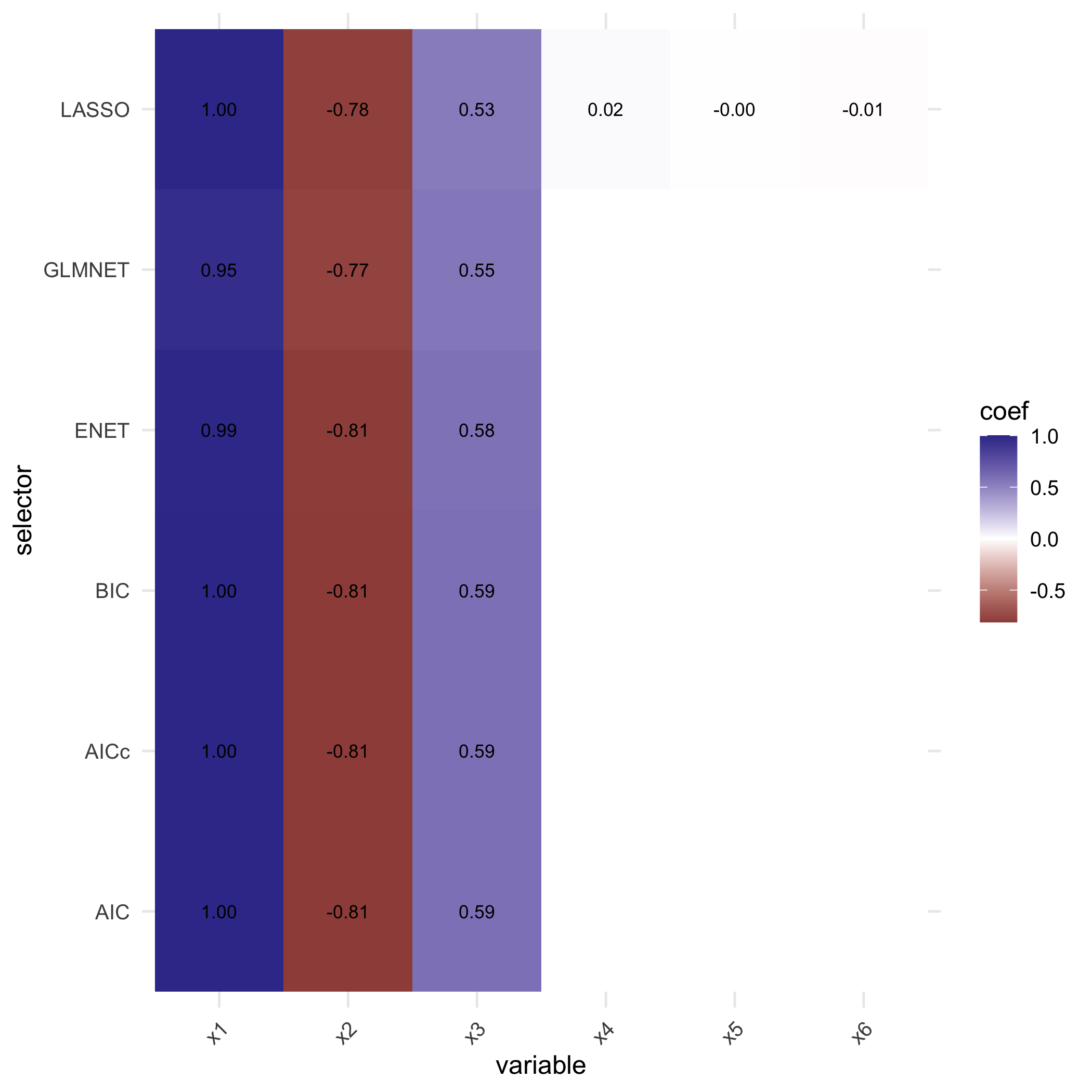
plot of chunk unnamed-chunk-8
plot_compare_freq(freq)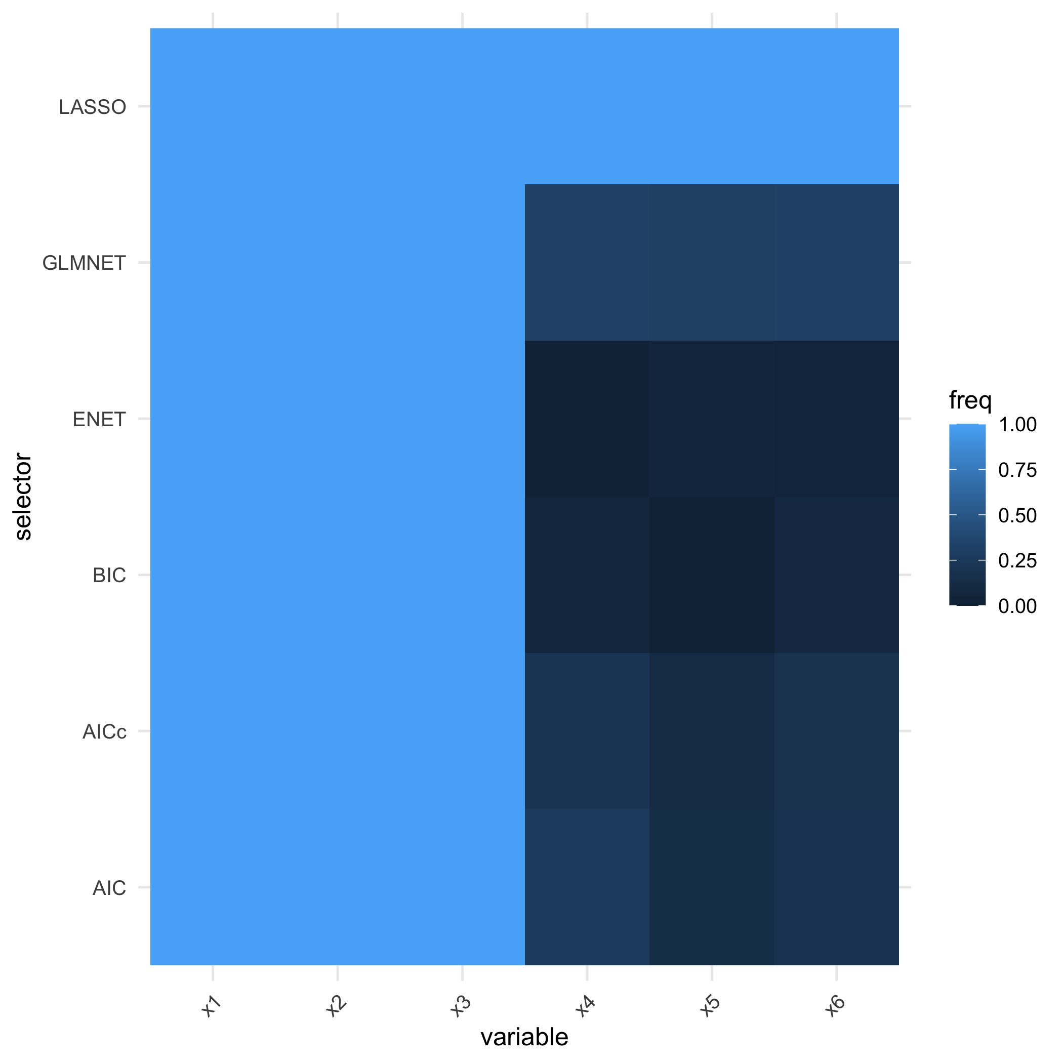
plot of chunk unnamed-chunk-9
sb_beta() can draw pseudo-responses from observed
intervals by supplying Y_low, Y_high, and an
interval mode:
interval_fit <- sb_beta(
  sim$X,
  Y_low = pmax(sim$Y - 0.05, 0),
  Y_high = pmin(sim$Y + 0.05, 1),
  interval = "uniform",
  B = 30,
  step.num = 0.5
)
attr(interval_fit, "interval")
#> [1] "uniform"
attr(interval_fit, "resample_diagnostics")
#> $`c0 = 1.000`
#> [1] group                   size                    regenerated             cached
#> [5] mean_abs_corr_orig      mean_abs_corr_surrogate mean_abs_corr_cross
#> <0 rows> (or 0-length row.names)
#>
#> $`c0 = 0.059`
#>            group size regenerated cached mean_abs_corr_orig mean_abs_corr_surrogate mean_abs_corr_cross
#> 1    x1,x2,x3,x4    4          30  FALSE         0.06136428              0.08465482          0.06242124
#> 2 x1,x2,x3,x5,x6    5          30  FALSE         0.06152013              0.08852213          0.07072896
#> 3    x1,x2,x3,x5    4          30  FALSE         0.07198271              0.09486290          0.06465764
#> 4       x1,x4,x5    3          30  FALSE         0.06290784              0.08437581          0.07146798
#> 5    x2,x3,x4,x5    4          30  FALSE         0.05766823              0.07919466          0.07095218
#> 6          x2,x6    2          30  FALSE         0.10556609              0.11117186          0.06506660
#>
#> $`c0 = 0.000`
#>               group size regenerated cached mean_abs_corr_orig mean_abs_corr_surrogate mean_abs_corr_cross
#> 1 x1,x2,x3,x4,x5,x6    6          30  FALSE         0.05666305              0.08767186           0.0650419
For a shortcut that always uses interval resampling, call
sb_beta_interval(sim$X, Y_low, Y_high, sample = "uniform").
The lower-level fastboost_interval() helper remains
available when you want to pair the interval resampling logic with a
custom selector outside sb_beta().
All selectors operate on responses in (0, 1). By default
sb_beta() and the selector helpers squeeze the data away
from the boundaries using the usual SelectBoost transformation. Set
squeeze = FALSE only if you have already applied your own
transformation; otherwise zero/one observations will trigger an
error.
Setting use.parallel = TRUE instructs
sb_beta() and sb_resample_groups() to dispatch
resamples and selector fits through future.apply.
Bring your own future::plan() to select the desired backend
(e.g. multisession on desktops):
future::plan(future::multisession)
sb_parallel <- sb_beta(sim$X, sim$Y, B = 50, step.num = 0.25, use.parallel = TRUE)
future::plan(future::sequential)
Refer to the vignettes for a more detailed walk-through of the
workflow and the pseudo-code underpinning the algorithms. The new
Getting started with SelectBoost.beta vignette mirrors the
CRAN submission example set by showing a full run, interpreting the
stability matrix, and comparing selectors side by side.
These binaries (installable software) and packages are in development.
They may not be fully stable and should be used with caution. We make no claims about them.