The hardware and bandwidth for this mirror is donated by METANET, the Webhosting and Full Service-Cloud Provider.
If you wish to report a bug, or if you are interested in having us mirror your free-software or open-source project, please feel free to contact us at mirror[@]metanet.ch.
The goal of affinitymatrix is to provide a set of tools
to estimate matching models without frictions and with Transferable
Utility starting from matched data. The package contains a set of
functions to implement the tools developed by Dupuy and Galichon (2014),
Dupuy, Galichon and Sun (2019) and Ciscato, Galichon and Gousse
(2020).
estimate.affinity.matrix estimates the affinity
matrix of the matching model of Dupuy and Galichon (2014), performs the
saliency analysis and the rank tests. The user must supply a matched
sample that is treated as the equilibrium matching of a bipartite
one-to-one matching model without frictions and with Transferable
Utility. For the sake of clarity, in the documentation we take the
example of the marriage market and refer to “men” as the observations on
one side of the market and to “women” as the observations on the other
side. Other applications may include matching between CEOs and firms,
firms and workers, buyers and sellers, etc. An example is provided
below.
estimate.affinity.matrix.lowrank estimates the
affinity matrix of the matching model of Dupuy and Galichon (2014) under
a rank restriction on the affinity matrix, as suggested by Dupuy,
Galichon and Sun (2019). In their own words, “to accommodate high
dimensionality of the data, they propose a novel method that
incorporates a nuclear norm regularization which effectively enforces a
rank constraint on the affinity matrix.” This function also performs the
saliency analysis and the rank tests. This function is a potential
alternative to estimate.affinity.matrix when the number of
matching variables is low relatively to the number of observed matches
or when the researcher believes that the number of dimensions of the
matching problem is much lower than the number of observed variables
considered.
estimate.affinity.matrix.unipartite estimates the
affinity matrix of the matching model of Ciscato, Gousse and Galichon
(2020), performs the saliency analysis and the rank tests. The model is
called unipartite (otherwise known as the “roommate problem”) and
differs from the original Dupuy and Galichon (2014) since all agents are
pooled in one group and can match within the group. For the sake of
clarity, in the documentation we take the example of the same-sex
marriage market and refer to “first partner” and “second partner” in
order to distinguish between the arbitrary partner order in a database
(e.g., survey respondent and partner of the respondent). Note that in
this case the variable “sex” is treated as a matching variable rather
than a criterion to assign partners to one side of the market as in the
bipartite case. Other applications may include matching between
coworkers, roommates or teammates.
You can install the released version of affinitymatrix
directly from Github
with:
devtools::install_github("edoardociscato/affinitymatrix")The example below shows how to use the main function of the package,
estimate.affinity.matrix, and how to summarize its
findings. We first generate a random sample of matches: the
values of the normalized variance-covariance matrix used in the data
generating process are taken from Chiappori, Ciscato and Guerriero
(2020). For the sake of clarity, consider the marriage market example:
every row of our data frame corresponds to a couple. The first
Kx columns correspond to the husbands’ characteristics, or
matching variables, while the last Ky columns
correspond to the wives’. The key inputs to feed to
estimate.affinity.matrix are two matrices X
and Y corresponding to the husbands’ and wives’ traits and
sorted so that the i-th man in X is married to the i-th
woman in Y.
# Load
library(affinitymatrix)

# Parameters
Kx = 4; Ky = 4; # number of matching variables on both sides of the market
N = 100 # sample size
mu = rep(0, Kx+Ky) # means of the data generating process
Sigma = matrix(c(1, 0.326, 0.1446, -0.0668, 0.5712, 0.4277, 0.1847, -0.2883, 0.326, 1, -0.0372, 0.0215, 0.2795, 0.8471, 0.1211, -0.0902, 0.1446, -0.0372, 1, -0.0244, 0.2186, 0.0636, 0.1489, -0.1301, -0.0668, 0.0215, -0.0244, 1, 0.0192, 0.0452, -0.0553, 0.2717, 0.5712, 0.2795, 0.2186, 0.0192, 1, 0.3309, 0.1324, -0.1896, 0.4277, 0.8471, 0.0636, 0.0452, 0.3309, 1, 0.0915, -0.1299, 0.1847, 0.1211, 0.1489, -0.0553, 0.1324, 0.0915, 1, -0.1959, -0.2883, -0.0902, -0.1301, 0.2717, -0.1896, -0.1299, -0.1959, 1),
               nrow=Kx+Ky) # (normalized) variance-covariance matrix of the data generating process
labels_x = c("Educ.", "Age", "Height", "BMI") # labels for men's matching variables
labels_y = c("Educ.", "Age", "Height", "BMI") # labels for women's matching variables

# Sample
data = MASS::mvrnorm(N, mu, Sigma) # generating sample
X = data[,1:Kx]; Y = data[,Kx+1:Ky] # men's and women's sample data
w = sort(runif(N-1)); w = c(w,1) - c(0,w) # sample weights

# Main estimation
res = estimate.affinity.matrix(X, Y, w = w, nB = 500)
#> Setup...
#> Main estimation...
#> Saliency analysis...
#> Rank tests...
#> Saliency analysis (bootstrap)...
The output of estimate.affinity.matrix is a list of
objects that constitute the estimation results. The estimated affinity
matrix is stored under Aopt, while the vector of loadings
describing men’s and women’s matching factors are stored under
U and V respectively. The following functions
can be used to produce summaries of the different findings. For further
details, Chiappori, Ciscato and Guerriero (2020) contain tables and
plots that are generated with these functions.
# Print affinity matrix with standard errors
table1 = show.affinity.matrix(res, labels_x = labels_x, labels_y = labels_y)
# Here we print a Markdown version: we recommend using the function export.table to store the tables in a txt file
# export.table(table1, name = "affinity_matrix", "path = "myresults")
gsub("\\}", "***", gsub("\\\\|hline|textbf\\{|\t|&|\n", "", table1))
#> [,1] [,2] [,3] [,4] [,5]
#> [1,] "" "Educ." "Age" "Height" "BMI"
#> [2,] "Educ." "1.12***" "0.39" "0.08" "-0.45***"
#> [3,] "" "(0.25) " "(0.34) " "(0.18) " "(0.18) "
#> [4,] "Age" "-0.52" "4.48***" "0.98***" "0.69***"
#> [5,] "" "(0.35) " "(0.71) " "(0.29) " "(0.28) "
#> [6,] "Height" "0.15" "0.41" "0.10" "-0.12"
#> [7,] "" "(0.17) " "(0.26) " "(0.13) " "(0.13) "
#> [8,] "BMI" "0.78***" "0.14" "0.10" "0.07"
#> [9,] "" "(0.19) " "(0.27) " "(0.14) " "(0.14) "
# Print diagonal elements of the affinity matrix with standard errors
table2 = show.diagonal(res, labels = labels_x)
# export.table(table2, name = "diagonal_affinity_matrix", "path = "myresults")
gsub("\\}", "***", gsub("\\\\|hline|textbf\\{|\t|&|\n", "", table2))
#> [,1] [,2] [,3] [,4]
#> [1,] "Educ." "Age" "Height" "BMI"
#> [2,] "1.12***" "4.48***" "0.10" "0.07"
#> [3,] "(0.25)" "(0.71)" "(0.13)" "(0.14)"
# Print rank test summary
table3 = show.test(res)
# export.table(table3, name = "rank_tests", "path = "myresults")
gsub("\\}", "***", gsub("\\\\|hline|textbf\\{|\t|&|\n", "", table3))
#> [,1] [,2] [,3] [,4]
#> [1,] "$H_0$: $rk(A)=k$" "$k=1$" "$k=2$" "$k=3$"
#> [2,] "$chi^2$" "36.55" "6.62" "0.06"
#> [3,] "$df$" "9" "4" "1"
#> [4,] "Rejected?" "Yes" "No" "No"
# Print results from saliency analysis
table4 = show.saliency(res, labels_x = labels_x, labels_y = labels_y, ncol_x = 2, ncol_y = 2)
# export.table(table4$U.table, name = "saliency_men", "path = "myresults")
# export.table(table4$V.table, name = "saliency_women", "path = "myresults")
gsub("\\}", "***", gsub("\\\\|hline|textbf\\{|\t|&|\n|$", "", table4$U.table))
#> [,1] [,2] [,3]
#> [1,] "" "Index 1" "Index 2"
#> [2,] "Educ." "0.05" "0.85***"
#> [3,] "Age" "1.00***" "-0.06***"
#> [4,] "Height" "0.08" "0.16"
#> [5,] "BMI" "0.02" "0.51***"
#> [6,] " Index share" "0.72" "0.22"
gsub("\\}", "***", gsub("\\\\|hline|textbf\\{|\t|&|\n|$", "", table4$V.table))
#> [,1] [,2] [,3]
#> [1,] "" "Index 1" "Index 2"
#> [2,] "Educ." "-0.09***" "0.95***"
#> [3,] "Age" "0.96***" "0.12***"
#> [4,] "Height" "0.21***" "0.05"
#> [5,] "BMI" "0.14***" "-0.28***"
#> [6,] " Index share" "0.72" "0.22"
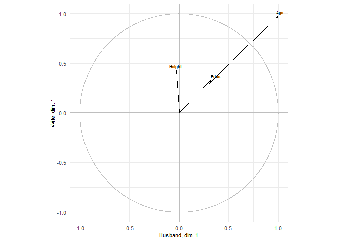
# Show correlation between observed variables and matching factors
plots = show.correlations(res, labels_x = labels_x, labels_y = labels_y,
label_x_axis = "Husband", label_y_axis = "Wife")
# for (d in 1:length(plots)) ggsave(paste0("myresults/plot_",d) plot = plots[d])
plots[1]
#> [[1]]
plots[2]
#> [[1]]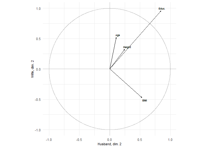
Ciscato, Edoardo, Alfred Galichon, and Marion Gousse. “Like attract like? a structural comparison of homogamy across same-sex and different-sex households.” Journal of Political Economy 128, no. 2 (2020): 740-781.
Chiappori, Pierre-André, Edoardo Ciscato, and Carla Guerriero. “Analyzing matching patterns in marriage: theory and application to Italian data.” HCEO Working Paper no. 2020-080 (2020).
Dupuy, Arnaud, and Alfred Galichon. “Personality traits and the marriage market.” Journal of Political Economy 122, no. 6 (2014): 1271-1319.
Dupuy, Arnaud, Alfred Galichon, and Yifei Sun. “Estimating matching affinity matrices under low-rank constraints.” Information and Inference: A Journal of the IMA 8, no. 4 (2019): 677-689.
These binaries (installable software) and packages are in development.
They may not be fully stable and should be used with caution. We make no claims about them.