The hardware and bandwidth for this mirror is donated by METANET, the Webhosting and Full Service-Cloud Provider.
If you wish to report a bug, or if you are interested in having us mirror your free-software or open-source project, please feel free to contact us at mirror[@]metanet.ch.

cdtr

Constrained Delaunay triangulation with refinement for R, binding the header-only CDT library (MPL-2.0). It takes the same input as a planar straight line graph (vertices, segments as index pairs, optional per-vertex attributes) and returns vertices, triangles, and a per-triangle depth that says where each triangle sits relative to the constraints, with no point-in-polygon step.

remotes::install_github("hypertidy/cdtr")

The pipeline, on a toy

Vertices and segments in, vertices and triangles out. Here a square with a square hole: two closed rings of segments.

library(cdtr)
x <- c(0, 1, 1, 0, 0.25, 0.75, 0.75, 0.25)
y <- c(0, 0, 1, 1, 0.25, 0.25, 0.75, 0.75)
s0 <- 1:8; s1 <- c(2, 3, 4, 1, 6, 7, 8, 5)
r <- cdt_triangulate(x, y, s0, s1)
str(r[c("P", "T", "S", "depth")])
#> List of 4
#>  $ P    : num [1:8, 1:2] 0 1 1 0 0.25 0.75 0.75 0.25 0 0 ...
#>  $ T    : int [1:10, 1:3] 8 6 8 7 6 5 8 6 2 2 ...
#>  $ S    : int [1:8, 1:2] 1 3 1 5 6 2 7 5 2 4 ...
#>  $ depth: int [1:10] 2 1 1 1 2 1 1 1 1 1

depth is the number of constraint boundaries crossed on the way in from outside: 0 is outside everything, and for nested rings odd is inside, even is a hole. By default triangles outside the outermost boundary are already dropped (erase = "outer", which is what Triangle’s -p does); erase = "holes" also drops the even depths.

plot_mesh <- function(m, main = "") {
  e <- cdt_edges(m)
  plot(m$P, asp = 1, axes = FALSE, xlab = "", ylab = "", pch = ".", main = main)
  segments(m$P[e[, 1], 1], m$P[e[, 1], 2], m$P[e[, 2], 1], m$P[e[, 2], 2], col = "grey50")
  segments(m$P[m$S[, 1], 1], m$P[m$S[, 1], 2], m$P[m$S[, 2], 1], m$P[m$S[, 2], 2], lwd = 2)
}
op <- par(mfrow = c(1, 3), mar = c(0.5, 0.5, 2, 0.5))
plot_mesh(r, "constrained")
plot_mesh(cdt_triangulate(x, y, s0, s1, max_area = 0.01), "max_area = 0.01")
plot_mesh(cdt_triangulate(x, y, s0, s1, max_area = 0.01, min_angle = 25, erase = "holes"),
          "+ min_angle = 25, holes erased")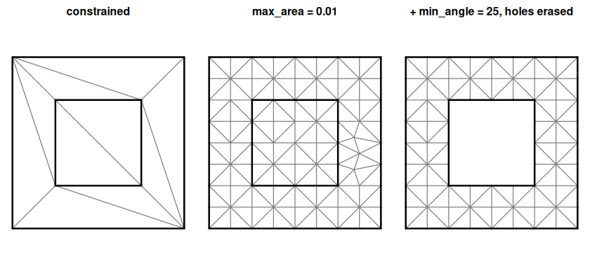

par(op)

Refinement reports what it could not do

Ruppert refinement cannot always meet the bound (two constraints meeting at a sharp angle, say). Rather than silently stopping, the result carries the counts.

r2 <- cdt_triangulate(x, y, s0, s1, max_area = 0.01, min_angle = 25)
r2$unrefined
#>   criterion shortEdgeTriangles circumcenterOutside circumcenterOnVertex
#> 1      area                  0                   0                    0
#> 2     angle                  0                   0                    0
#>   sharpFixedCorner shortEdges splitVertexInvalid
#> 1                0          0                  0
#> 2                0          0                  0
r2$min_edge_length
#> [1] 0.025

min_edge_length is the floor below which the refiner gives up on an edge; by default it is derived from the input (a fraction of the median segment length, capped by the area target) so refinement does not cascade into sharp input corners. Pass 0 for never-give-up.

Real polygons

Any polygon source reduces to the same two tables. With sf’s North Carolina counties, rings become vertex runs and consecutive index pairs; shared boundaries dedupe to one segment.

nc <- sf::st_read(system.file("shape/nc.shp", package = "sf"), quiet = TRUE)
rings <- unlist(lapply(sf::st_geometry(nc), function(g) lapply(unclass(g), `[[`, 1)), recursive = FALSE)
xy <- do.call(rbind, lapply(rings, function(m) m[-nrow(m), ]))
n <- vapply(rings, function(m) nrow(m) - 1L, 1L)
start <- rep(cumsum(c(0L, n[-length(n)])), n)
s0 <- seq_along(xy[, 1])
s1 <- start + (s0 - start) %% rep(n, n) + 1L
m <- cdt_triangulate(xy[, 1], xy[, 2], s0, s1, max_area = 0.01)
table(m$depth)
#> 
#>    1    3    5 
#> 2100 1119  521
op <- par(mar = rep(0, 4))
plot_mesh(m)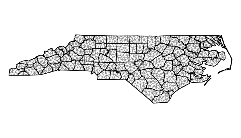

par(op)

The counties tile the state, so there are no holes, but a county two boundaries in from the coast has depth 3, and so on: depth is the peel layer, a count of constraint crossings from outside, not an inside/outside flag in general. It is computed topologically from the mesh alone, before anything is erased, which makes it a cheap first cut for classifying triangles by region: nested rings get odd/even, a coverage gets a boundary-distance ordering, and only ties within a layer need a geometric lookup.

Attributes ride along

Per-vertex values (an elevation, a time) are carried onto the new Steiner vertices by linear interpolation from the input mesh, the way Triangle’s PA works.

z <- 2 * xy[, 1] + 3 * xy[, 2]
ma <- cdt_triangulate_attr(xy[, 1], xy[, 2], s0, s1, PA = cbind(z = z), max_area = 0.01)
range(ma$PA[, "z"] - (2 * ma$P[, 1] + 3 * ma$P[, 2]))
#> [1] -1.421085e-14  1.421085e-14

What this is for

cdtr is the triangulation primitive for the hypertidy mesh packages, where it replaces RTriangle (Shewchuk’s Triangle, non-commercial licence). The inst/benchmarks/ scripts compare the two on anglr’s Tasmanian contour and cadastre data; the short version is that constrained-only output is identical, refinement honours max_area where Triangle may give up, and Triangle’s refiner is faster per Steiner point.

These binaries (installable software) and packages are in development.
They may not be fully stable and should be used with caution. We make no claims about them.