The hardware and bandwidth for this mirror is donated by METANET, the Webhosting and Full Service-Cloud Provider.
If you wish to report a bug, or if you are interested in having us mirror your free-software or open-source project, please feel free to contact us at mirror[@]metanet.ch.
![]()
![]()
The {choicedata} package simplifies working with choice
data in R.
The package breaks down the process of modeling choice data into a series of steps. Each step is represented by an object that contains the necessary information for the subsequent step.
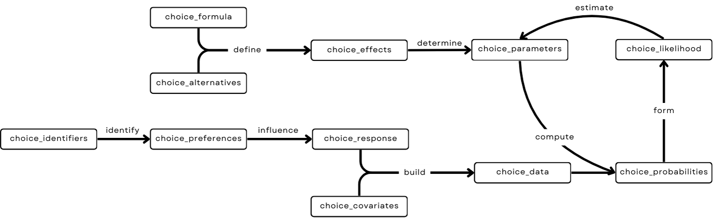
choice_formula:
the choice model formula.
choice_alternatives:
the set of choice alternatives.
choice_effects:
the choice effects, defined by choice_alternatives and
choice_formula.
choice_parameters:
the model parameters, determined by choice_effects and
estimated via choice_likelihood.
choice_identifiers:
the identifiers for deciders and choice occasions.
choice_preferences:
the deciders’ choice preferences, identified by
choice_identifiers.
choice_responses:
the choice responses, influenced by
choice_preferences.
choice_covariates:
the choice covariates.
choice_data:
the choice data, built by choice_covariates and
choice_responses.
choice_probabilities:
the choice probabilities, computed from choice_data and
choice_parameters.
choice_likelihood:
the likelihood of the choice model, formed by
choice_probabilities.
The objects are designed to be modular and can be combined in various ways to create a range of modeling workflows.
The travel_mode_choice data set contains the revealed
preferences of 210 travelers choosing between plane, train, bus, and
car. We can transform the data from long to wide format, or construct
model design matrices:
library("choicedata")

travel_mode_choice
#> # A tibble: 840 × 8
#>    individual mode  choice  wait  cost travel income  size
#>         <int> <chr>  <int> <int> <int>  <int>  <int> <int>
#>  1          1 plane      0    69    59    100     35     1
#>  2          1 train      0    34    31    372     35     1
#>  3          1 bus        0    35    25    417     35     1
#>  4          1 car        1     0    10    180     35     1
#>  5          2 plane      0    64    58     68     30     2
#>  6          2 train      0    44    31    354     30     2
#>  7          2 bus        0    53    25    399     30     2
#>  8          2 car        1     0    11    255     30     2
#>  9          3 plane      0    69   115    125     40     1
#> 10          3 train      0    34    98    892     40     1
#> # ℹ 830 more rows

long_to_wide(
  data_frame = travel_mode_choice,
  column_alternative = "mode",
  column_decider = "individual"
)
#> # A tibble: 210 × 16
#>    individual income  size wait_plane wait_train wait_bus wait_car cost_plane
#>         <int>  <int> <int>      <int>      <int>    <int>    <int>      <int>
#>  1          1     35     1         69         34       35        0         59
#>  2          2     30     2         64         44       53        0         58
#>  3          3     40     1         69         34       35        0        115
#>  4          4     70     3         64         44       53        0         49
#>  5          5     45     2         64         44       53        0         60
#>  6          6     20     1         69         40       35        0         59
#>  7          7     45     1         45         34       35        0        148
#>  8          8     12     1         69         34       35        0        121
#>  9          9     40     1         69         34       35        0         59
#> 10         10     70     2         69         34       35        0         58
#> # ℹ 200 more rows
#> # ℹ 8 more variables: cost_train <int>, cost_bus <int>, cost_car <int>,
#> #   travel_plane <int>, travel_train <int>, travel_bus <int>, travel_car <int>,
#> #   choice <chr>

mode_effects <- choice_effects(
  choice_formula = choice_formula(
    formula = choice ~ cost | income + size | travel + wait,
    error_term = "probit"
  ),
  choice_alternatives = choice_alternatives(
    J = 4,
    alternatives = unique(travel_mode_choice$mode)
  )
)

mode_data <- choice_data(
  data_frame = travel_mode_choice,
  format = "long",
  column_choice = "choice",
  column_decider = "individual",
  column_alternative = "mode",
  column_ac_covariates = c("income", "size"),
  column_as_covariates = c("wait", "cost", "travel")
)

design_matrices <- design_matrices(mode_data, mode_effects)
design_matrices[[1]]
#>       cost income_car income_plane income_train size_car size_plane size_train
#> bus     25          0            0            0        0          0          0
#> car     10         35            0            0        1          0          0
#> plane   59          0           35            0        0          1          0
#> train   31          0            0           35        0          0          1
#>       ASC_car ASC_plane ASC_train travel_bus travel_car travel_plane
#> bus         0         0         0        417          0            0
#> car         1         0         0          0        180            0
#> plane       0         1         0          0          0          100
#> train       0         0         1          0          0            0
#>       travel_train wait_bus wait_car wait_plane wait_train
#> bus              0       35        0          0          0
#> car              0        0        0          0          0
#> plane            0        0        0         69          0
#> train 372 0 0 0 34generate_choice_data() makes it straightforward to
simulate choice data. The example below simulates 200 ranking tasks with
three alternatives and recovers the data-generating parameters via
numerical optimization of the likelihood:
library("choicedata")

set.seed(1)

sim_effects <- choice_effects(
  choice_formula = choice_formula(
    formula = choice ~ A | B | C,
    error_term = "logit"
  ),
  choice_alternatives = choice_alternatives(
    J = 3,
    alternatives = c("A", "B", "C")
  )
)

sim_parameters <- generate_choice_parameters(sim_effects)

(sim_data <- generate_choice_data(
  choice_effects = sim_effects,
  choice_identifiers = generate_choice_identifiers(N = 200),
  choice_parameters = sim_parameters,
  choice_type = "ranked"
))
#> # A tibble: 200 × 13
#>    deciderID occasionID choice        B choice_A choice_B choice_C     A_A
#>  * <chr>     <chr>      <chr>     <dbl>    <int>    <int>    <int>   <dbl>
#>  1 1         1          B       1.12           2        1        3  0.576
#>  2 2         1          B       0.782          3        1        2 -0.0449
#>  3 3         1          B      -0.478          2        1        3  0.0746
#>  4 4         1          B      -0.415          3        1        2  0.418
#>  5 5         1          B       0.697          2        1        3 -0.394
#>  6 6         1          B       0.881          2        1        3  0.557
#>  7 7         1          B      -0.367          3        1        2  0.398
#>  8 8         1          B       0.0280         3        1        2 -1.04
#>  9 9         1          C       0.476          3        2        1 -0.743
#> 10 10        1          B       0.00111        2        1        3 -0.710
#> # ℹ 190 more rows
#> # ℹ 5 more variables: A_B <dbl>, A_C <dbl>, C_A <dbl>, C_B <dbl>, C_C <dbl>

sim_likelihood <- choice_likelihood(
  choice_data = sim_data,
  choice_effects = sim_effects
)

objective <- sim_likelihood$objective
true_vector <- switch_parameter_space(
  choice_parameters = sim_parameters,
  choice_effects = sim_effects
)

fit <- stats::optim(
  par = stats::rnorm(length(true_vector)),
  fn = function(par) {
    objective(choice_parameters = par, logarithm = TRUE, negative = TRUE)
  }
)

estimated_parameters <- switch_parameter_space(
  choice_parameters = fit$par,
  choice_effects = sim_effects
)

data.frame(dgp = true_vector, estimated = fit$par)
#>               dgp   estimated
#> beta_1 -1.9810209 -2.04179163
#> beta_2  0.5807312  0.04789289
#> beta_3 -2.6424897 -3.05406623
#> beta_4  5.0447208  4.82873952
#> beta_5  1.0419951  0.99061141
#> beta_6 -2.5945488 -2.75745549
#> beta_7  1.5413860  1.21554512
#> beta_8 2.3347877 1.96729481You can install the released package version from CRAN with:
install.packages("choicedata"){Rprobit} (Bauer et
al. 2023) provides maximum approximated composite marginal
likelihood estimation for efficient probit choice modeling.
{RprobitB} (Oelschläger
and Bauer 2025) provides Bayesian tools for estimating probit
models.
You have a question, found a bug, request a feature, want to give feedback, or like to contribute? Please file an issue on GitHub.
These binaries (installable software) and packages are in development.
They may not be fully stable and should be used with caution. We make no claims about them.