The hardware and bandwidth for this mirror is donated by METANET, the Webhosting and Full Service-Cloud Provider.
If you wish to report a bug, or if you are interested in having us mirror your free-software or open-source project, please feel free to contact us at mirror[@]metanet.ch.
The goal of ciccr is to implement methods for carrying out causal inference in case-control and case-population studies (Jun and Lee, 2023).
You can install the released version of ciccr from CRAN with:
install.packages("ciccr")Alternatively, you can install the development version from GitHub with:
# install.packages("devtools") # uncomment this line if devtools is not installed yet
devtools::install_github("sokbae/ciccr")We first call the ciccr package.
library(ciccr)To illustrate the usefulness of the package, we use the dataset ACS_CC that is included the package. This dataset is an extract from American Community Survey (ACS) 2018, restricted to white males residing in California with at least a bachelor’s degree. The ACS is an ongoing annual survey by the US Census Bureau that provides key information about US population. We use the following variables:
  y = ACS_CC$topincome
  t = ACS_CC$baplus
  x = ACS_CC$age
The binary outcome y is defined to be one if a
respondent’s annual total pre-tax wage and salary income is top-coded.
In the sample extract, the top-coded income bracket has median income
$565,000 and the next highest income that is not top-coded is
$327,000.
The binary treatment t is defined to be one if a
respondent has a master’s degree, a professional degree, or a doctoral
degree.
The covariate x is age in years and is restricted to
be between 25 and 70.
The original ACS survey is not from case-control sampling but we construct a case-control sample by the following procedure:
We now construct cubic b-spline terms with three inner knots using the age variable.
x = splines::bs(x, df = 6)Using the retrospective sieve logistic regression model, we estimate the average of the log odds ratio conditional on the case sample by
  results_case = avg_RR_logit(y, t, x, 'case')
  results_case$est
#>         y
#> 0.7286012
  results_case$se
#>         y
#> 0.1013445
Here, option 'case' refers to conditioning on the event
that income is top-coded.
Similarly, we estimate the average of the log odds ratio conditional on the control sample by
  results_control = avg_RR_logit(y, t, x, 'control')
  results_control$est
#>         y
#> 0.5469094
  results_control$se
#>         y
#> 0.1518441
Here, option 'control' refers to conditioning on the
event that income is not top-coded.
We carry out causal inference by
results = cicc_RR(y, t, x, 'cc', 0.95)Here, ‘cc’ refers to case-control sampling and 0.95 refers to the level of the uniform confidence band (0.95 is the default choice).
  est = results$est
  print(est)
#>         y         y
#> 0.5469094 0.7286012
  se = results$se
  print(se)
#>         y         y
#> 0.1518441 0.1013445
  ci = results$ci
  print(ci)
#>         y         y
#> 0.8445183 1.0262101
The S3 object results contains estimates
est, standard errors se, and one-sided
confidence bands ci at p = 0 and
p = 1. The point estimates and confidence interval
estimates of the cicc_RR command are based on the scale of
log relative risk. It is more conventional to look at the results in
terms of relative risk. To do so, we plot the results in the following
way:
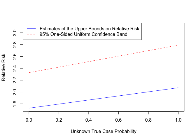
cicc_plot(results)
To interpret the results, we assume both marginal treatment response (MTR) and marginal treatment selection (MTS). In this setting, MTR means that everyone will not earn less by obtaining a degree higher than bachelor’s degree; MTS indicates that those who selected into higher education have higher potential to earn top incomes. Based on the MTR and MTS assumptions, we can conclude that the treatment effect lies in between 1 and the upper end point of the one-sided confidence interval with high probability. Thus, the estimates in the graph above suggest that the effect of obtaining a degree higher than bachelor’s degree is anywhere between 1 and the upper end points of the uniform confidence band. This roughly implies that the chance of earning top incomes may increase up to by a factor as large as the upper end points of the uniform confidence band, but allowing for possibility of no positive effect at all. The results are shown over the range of the unknown true case probability. See Jun and Lee, 2020 for more detailed explanations regarding how to interpret the estimation results.
We can compare these results with estimates obtained from logistic regression.
logit = stats::glm(y~t+x, family=stats::binomial("logit"))
est_logit = stats::coef(logit)
ci_logit = stats::confint(logit, level = 0.9)
#> Waiting for profiling to be done...
# point estimate
exp(est_logit)
#> (Intercept)           t          x1          x2          x3          x4
#>  0.05461156  2.06117153  4.42179639 12.99601849 19.03962976 26.83565737
#>          x5          x6
#>  6.42381406 26.14359394
# confidence interval
exp(ci_logit)
#>                     5 %       95 %
#> (Intercept)  0.01960819  0.1304108
#> t            1.75166056  2.4271287
#> x1           1.05679997 21.6604223
#> x2           5.50583091 33.8909622
#> x3           6.79458010 61.3258710
#> x4          10.22943808 78.7353953
#> x5           2.00536450 22.8509008
#> x6           8.66983039 87.6311482
Here, the relevant coefficient is 2.06 (t) and its
two-sided 90% confidence interval is [1.75, 2.43]. If we assume strong
ignorability, the treatment effect is about 2 and its two-sided
confidence interval is between [1.75, 2.43]. However, it is unlikely
that the higher-degrees-than-BA treatment satisfies the strong
ignorability condition.
See the vignette for other examples that include inference on attributable risk and how to work with case-population samples.
Jun, S.J. and Lee, S. (2023). Causal Inference under Outcome-Based Sampling with Monotonicity Assumptions. https://arxiv.org/abs/2004.08318, accepted for publication in Journal of Business & Economic Statistics.
Manski, C.F. (1997). Monotone Treatment Response. Econometrica, 65(6), 1311-1334.
Manski, C.F. and Pepper, J.V. (2000). Monotone Instrumental Variables: With an Application to the Returns to Schooling. Econometrica, 68(4), 997-1010.
These binaries (installable software) and packages are in development.
They may not be fully stable and should be used with caution. We make no claims about them.