The hardware and bandwidth for this mirror is donated by METANET, the Webhosting and Full Service-Cloud Provider.
If you wish to report a bug, or if you are interested in having us mirror your free-software or open-source project, please feel free to contact us at mirror[@]metanet.ch.

Visualization and Polytomous Modeling of Survival and Competing Risks with Minimal Code — cifmodeling

Are you comfortable writing Surv(time, status) ~ strata but hesitant to dive into the Fine-Gray models or custom ggplot2 code? cifmodeling helps clinicians, epidemiologists, and applied researchers move from basic Kaplan–Meier curves to clear, publication-ready survival and competing risk plots – with just a few lines of R.

This package provides a unified, high-level interface for survival and competing-risks analysis, combining nonparametric estimation, regression modeling, and visualization. It is centered around three tightly connected functions:

• cifplot() generates a survival or cumulative incidence function (CIF) curve. The visualization is built on top of ggsurvfit and ggplot2.
• cifpanel() creates multi-panel displays for survival/CIF curves, arranged either in a grid layout or as an inset overlay.
• polyreg() fits coherent regression models on all cause-specific CIFs simultaneously.

Explore the main features visually:
See the Gallery for a curated set of examples using cifplot() and cifpanel().

Learn the modeling framework with polyreg():
See the Direct polytomous regression for coherent, joint modeling of all cause-specific CIFs.

Quick start

library(cifmodeling)
data(diabetes.complications)
cifplot(Event(t,epsilon)~fruitq, data=diabetes.complications, 
        outcome.type="competing-risk", panel.per.event=TRUE)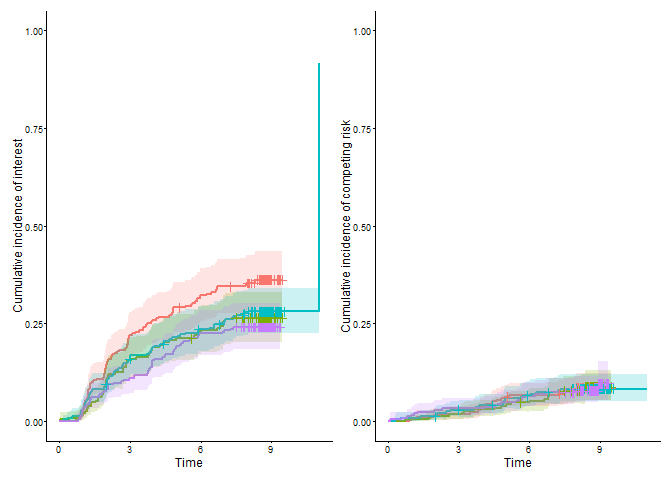

Aalen-Johansen cumulative incidence curves from cifplot()

In competing risks data, censoring is often coded as 0, the event of interest as 1, and competing risks as 2. In the diabetes.complications data frame, epsilon follows this convention. With panel.per.event = TRUE, cifplot() visualizes both competing events, with the CIF of diabetic retinopathy (epsilon = 1) shown on the left and the CIF of macrovascular complications (epsilon = 2) on the right.

A workflow of competing risks analysis

Four code snippets illustrate how the three core functions interact with existing resources and analyze complex competing risks data:

• Describe the competing risks via a CIF plot with marks
• Plot adjusted CIFs using inverse probability weights (IPW)
• Estimate risk ratios for all competing events at a clinically relevant time
• Visualize how risk ratios evolve over time

We use the diabetes.complications data throughout, focusing on diabetic retinopathy (event 1) and macrovascular complications (event 2), with the level of fruit intake, low (Q1) and high (Q2 to 4), as the exposure (fruitq1).

CIF plot with competing-risk marks

The first snippet is plotting the CIF of diabetic retinopathy with marks indicating individuals who experienced macrovascular complications first (add.competing.risk.mark = TRUE). Here we show a workflow slightly different from the code at the beginning. First, the time points at which the macrovascular complications occurred were obtained as output1 for each strata using a helper function extract_time_to_event(). Then, cifplot() is used to generate the figure. The label.y, label.x, label.strata and limit.x arguments are also used to customize the labels and axis limits.

data(diabetes.complications)
output1 <- extract_time_to_event(Event(t,epsilon)~fruitq1, 
                                 data=diabetes.complications, which.event="event2")
cifplot(Event(t,epsilon)~fruitq1, data=diabetes.complications, 
        outcome.type="competing-risk",
        add.conf=FALSE, add.risktable=FALSE, add.censor.mark=FALSE,
        add.competing.risk.mark=TRUE, competing.risk.time=output1,
        label.y="CIF of diabetic retinopathy", label.x="Years from registration",
        limits.x=c(0,8), label.strata=c("High intake","Low intake"), 
        level.strata=c(0, 1), order.strata=c(0, 1))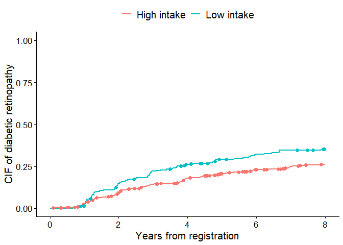

Cumulative incidence curves with competing-risk marks

IPW-adjusted CIF with cifplot() and CBPS()

In an observational study, it is necessary to adjust for confounders in order to compare fruit intake levels. In the next example, we obtain IPWs from CBPS() and draw adjusted CIFs. It is important to note that in IPW analysis, the SEs output in the unweighted analysis are not necessarily valid. Among the SE methods selectable in cifplot() (Aalen-, delta-, and influence-function-type), simulations by Deng and Wang (2025) have shown that the influence-function based SE performs well. This snippet displays valid CIs in the plot by specifying error=“if” and add.conf=TRUE.

if (requireNamespace("CBPS", quietly = TRUE)) {
 library(CBPS)

 output2 <- CBPS(
  fruitq1 ~ age + sex + bmi + hba1c + diabetes_duration + drug_oha + drug_insulin
   + sbp + ldl + hdl + tg + current_smoker + alcohol_drinker + ltpa,
  data = diabetes.complications, ATT=0
 )
 diabetes.complications$ipw <- output2$weights
 cifplot(Event(t,epsilon)~fruitq1, data=diabetes.complications, 
         outcome.type="competing-risk", weights = "ipw", 
         add.conf=TRUE, add.risktable=FALSE, add.censor.mark=FALSE,
         label.y="CIF of diabetic retinopathy", label.x="Years from registration",
         limits.x=c(0,8), label.strata=c("High intake","Low intake"), 
         level.strata=c(0, 1), order.strata=c(0, 1), error = "if")
} else {
 plot.new()
 text(0.5, 0.5,
 "Install the 'CBPS' package to run this example.",
 cex = 0.9)
}

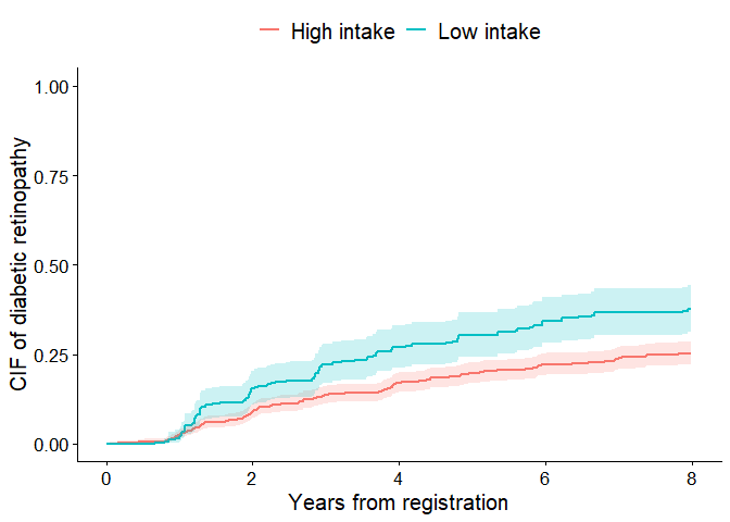
Adjusted cumulative incidence curves with CIs based on influence functions

Risk ratios for all competing events via polyreg()

We then fit polyreg() to estimate risk ratios for diabetic retinopathy and macrovascular complications, in a coherent joint model of all cause-specific CIFs at 8 years.

output3 <- polyreg(nuisance.model=Event(t,epsilon)~1, exposure="fruitq1", 
          data=diabetes.complications, effect.measure1="RR", effect.measure2="RR", 
          time.point=8, outcome.type="competing-risk")
summary(output3)
#> 
#>                       event1        event2      
#> ---------------------------------------------- 
#> fruitq1, 1 vs 0      
#>                       1.350         1.079       
#>                       [1.114, 1.637]  [0.682, 1.707]
#>                       (p=0.002)     (p=0.746)   
#> 
#> ---------------------------------------------- 
#> 
#> effect.measure        RR at 8       RR at 8     
#> n.events              279 in N = 978  79 in N = 978
#> median.follow.up      8             -           
#> range.follow.up       [0.05, 11.00]  -           
#> n.parameters          4             -           
#> converged.by          Converged in objective function  -           
#> nleqslv.message       Function criterion near zero  -

The summary() method prints an event-wise table of point estimates, CIs, and p-values. Internally, a "polyreg" object also supports the generics API:

• tidy(): coefficient-level summaries (one row per term and per event),
• glance(): model-level summaries (follow-up, convergence, number of events),
• augment(): observation-level diagnostics (weights for IPCW, predicted CIFs, and influence functions).

Risk ratios over time with modelplot()

Finally, we repeat the model at multiple time points and use modelplot() to visualize how risk ratios evolve over follow-up. With generics-Compatible objects, polyreg() is integrated naturally with the broader broom/modelsummary ecosystem. For publication-ready tables, you can pass polyreg objects directly to modelsummary::msummary() and modelsummary::modelplot(), including exponentiated summaries (risk ratios, odds ratios, subdistribution hazard ratios) via the exponentiate = TRUE option.

if (requireNamespace("modelsummary", quietly = TRUE)) {
 library(modelsummary)
 output4 <- polyreg(nuisance.model=Event(t,epsilon)~1, exposure="fruitq1", 
                    data=diabetes.complications, effect.measure1="RR", effect.measure2="RR", 
                    time.point=2, outcome.type="competing-risk")
 output5 <- polyreg(nuisance.model=Event(t,epsilon)~1, exposure="fruitq1", 
                    data=diabetes.complications, effect.measure1="RR", effect.measure2="RR", 
                    time.point=4, outcome.type="competing-risk")
 output6 <- polyreg(nuisance.model=Event(t,epsilon)~1, exposure="fruitq1", 
                    data=diabetes.complications, effect.measure1="RR", effect.measure2="RR", 
                    time.point=6, outcome.type="competing-risk")
 summary <- list(
  "RR of diabetic retinopathy at 2 years" = output4$summary$event1, 
  "RR of diabetic retinopathy at 4 years" = output5$summary$event1, 
  "RR of diabetic retinopathy at 6 years" = output6$summary$event1, 
  "RR of diabetic retinopathy at 8 years" = output3$summary$event1,
  "RR of macrovascular complications at 2 years" = output4$summary$event2, 
  "RR of macrovascular complications at 4 years" = output5$summary$event2, 
  "RR of macrovascular complications at 6 years" = output6$summary$event2, 
  "RR of macrovascular complications at 8 years" = output3$summary$event2
 )
 modelplot(summary, coef_rename="", exponentiate = TRUE)
} else {
 plot.new()
 text(0.5, 0.5,
 "Install the 'modelsummary' package to run this example.",
 cex = 0.9)
}

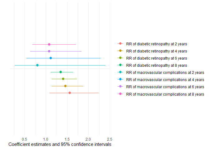
Visualizaton of risk ratios at 2, 4, 6 and 8 years using polyreg() and modelplot()

Why cifmodeling?

In clinical and epidemiologic research, analysts often need to handle censoring, competing risks, and intercurrent events (e.g. treatment switching), but existing R packages typically separate these tasks across different interfaces. cifmodeling provides a unified, publication-ready toolkit that integrates nonparametric estimation, regression modeling, and visualization for survival and competing risks data. The tools assist users in the following ways:

• Unified interface for the Kaplan–Meier and Aalen–Johansen curves, with survival and competing risks handled by the same Event() + formula + data syntax.
• Effects on the CIF scale: while the Fine-Gray models subdistribution hazards, polyreg() directly targets ratios of CIFs (risk ratios, odds ratios, subdistribution hazard ratios), so parameters align closely with differences seen in CIF curves.
• Coherent, joint modeling of all competing events: polyreg() models all cause-specific CIFs together, parameterizing the nuisance structure with polytomous log odds products and enforcing that their CIFs sum to at most one.
• Tidy summaries and reporting: support for generics::tidy(), glance(), and augment(), which integrate polyreg() smoothly with modelsummary and other broom-style tools.
• Publication-ready graphics built on ggsurvfit and ggplot2, including number-at-risk/CIF+CI tables, censoring/competing-risk/intercurrent-event marks, and multi-panel layouts.

Position in the survival ecosystem

Several excellent R packages exist for survival and competing risks analysis. The survival package provides the canonical API for survival data. In combination with the ggsurvfit package, survival::survfit() can produce publication-ready survival plots. For CIF plots, however, integration in the general ecosystem is less streamlined. cifmodeling fills this gap by offering cifplot() for survival/CIF plots and multi-panel figures via a single, unified interface.

Beyond providing a unified interface, cifcurve() also extends survfit() in a few targeted ways. For unweighted survival data, it reproduces the standard Kaplan-Meier estimator with Greenwood and Tsiatis SEs and a unified set of CI transformations. For competing risks data, it computes Aalen-Johansen CIFs with both Aalen-type and delta-method SEs. For weighted survival or competing risks data (e.g. inverse probability weighting), it implements influence-function based SEs (Deng and Wang 2025) as well as modified Greenwood- and Tsiatis-type SEs (Xie and Liu 2005), which are valid under general positive weights.

If you need very fine-grained plot customization, you can compute the estimator and keep a survfit-compatible object with cifcurve() (or supply your own survfit object) and then style it using ggsurvfit/ggplot2 layers. In other words:

• use cifcurve() for estimation,
• use cifplot() / cifpanel() for quick, high-quality figures, and
• fall back to the ggplot ecosystem when you want full artistic control.

The causalRisk focuses on causal cumulative risk and hazard estimation using IPW and related estimators. It allows users to specify treatment, outcome, censoring, and missingness models via a dedicated syntax (specify_models(), identify_*()), and then estimate counterfactual cumulative risks and risk differences/ratios under complex censoring and confounding structures, with built-in plotting and table-making utilities.

The mets package is a more specialized toolkit that provides advanced methods for competing risks analysis. cifmodeling::polyreg() focuses on coherent modeling of all CIFs simultaneously to estimate the exposure effects in terms of RR/OR/SHR. This coherence can come with longer runtimes for large problems. If you prefer fitting separate regression models for each competing event or specifically need the Fine-Gray models (Fine and Gray 1999) and the direct binomial models (Scheike, Zhang and Gerds 2008), mets::cifreg() and mets::binreg() are excellent choices.

Interested in the precise variance formulas and influence functions for the Aalen-Johansen estimator?
Visit Computational formulas in cifcurve().

Installation

The package is implemented in R and relies on Rcpp, nleqslv and boot for its numerical back-end. The examples in this document also use ggplot2, ggsurvfit, patchwork and modelsummary for tabulation and plotting. Install the core package and these companion packages with:

# Install cifmodeling from GitHub
devtools::install_github("gestimation/cifmodeling")

# Core dependencies
install.packages(c("Rcpp", "nleqslv", "boot"))

# Recommended packages for plotting and tabulation in this README
install.packages(c("ggplot2", "ggsurvfit", "patchwork", "modelsummary"))

Quality control

cifmodeling includes an extensive test suite built with testthat, which checks the numerical accuracy and graphical consistency of all core functions (cifcurve(), cifplot(), cifpanel(), and polyreg()). The estimators are routinely compared against related functions in survival, cmprsk and mets packages to ensure consistency. The package is continuously tested on GitHub Actions (Windows, macOS, Linux) to maintain reproducibility and CRAN-level compliance.

These binaries (installable software) and packages are in development.
They may not be fully stable and should be used with caution. We make no claims about them.