
The hardware and bandwidth for this mirror is donated by METANET, the Webhosting and Full Service-Cloud Provider.
If you wish to report a bug, or if you are interested in having us mirror your free-software or open-source project, please feel free to contact us at mirror[@]metanet.ch.
Rasterize geometry without materializing any pixel values. controlledburn produces sparse tables for polygon, line, and point input — one type-pure table per geometry kind.
Two modes: coverage (exact analytical coverage fractions via vendored exactextract math) and approx (cell-centre rule, fasterize semantics, runs only). Both are O(perimeter) in time and memory; no dense matrix is allocated.
Dependencies: cpp11, wk. No GEOS, no sf, no
Armadillo.
remotes::install_github("hypertidy/controlledburn")library(controlledburn)
library(geos)
poly <- as_geos_geometry("POLYGON ((1 1, 8.9 1, 8.9 9.12, 1 9.12, 1 1))")
# Coverage mode (default): exact boundary fractions
r <- burn(poly, extent = c(0, 10, 0, 10), dimension = c(20L, 20L))
r
#> <controlledburn> 20 x 20 grid, 1 geometry
#> runs: 45 (240 interior cells)
#> edges: 32 polygon boundary cells
#> sparsity: 32.0% empty
# Approx mode: cell-centre rule, runs only, no edges
r_approx <- burn(poly, extent = c(0, 10, 0, 10), dimension = c(20L, 20L),
mode = "approx")
r_approx
#> <controlledburn> 20 x 20 grid, 1 geometry
#> runs: 16 (256 interior cells)
#> edges: 0 polygon boundary cells
#> sparsity: 36.0% empty
# Materialize only when you need it
mat <- materialize_chunk(r)
ximage::ximage(mat, extent = c(0, 10, 0, 10), asp = 1)
plot(poly, add = TRUE)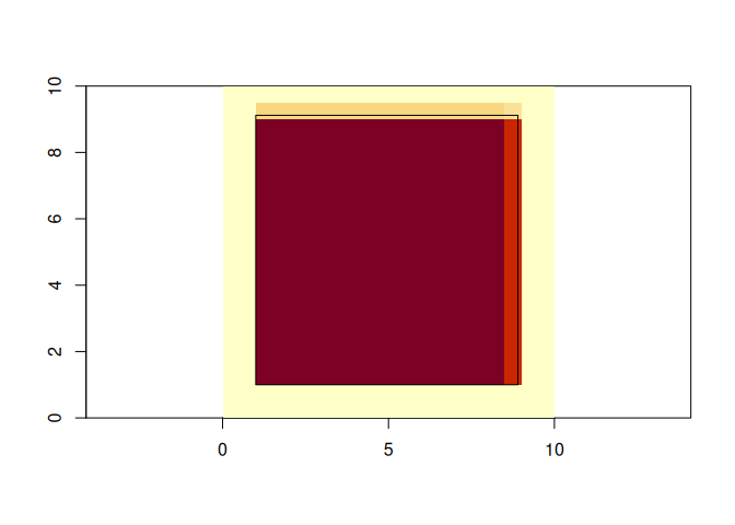
unique(c(mat))
#> [1] 0.000 0.240 1.000 0.192 0.800
## no variation in the approx mode
unique(c(materialise_chunk(r_approx)))
#> [1] 0 1With no extent or dimension, controlledburn derives both from the geometry:
r <- burn(poly)
# extent from wk::wk_bbox(), 256 cells on the long axis
Or specify resolution:
r <- burn(poly, resolution = 0.5)Lines produce a $lines table with absolute length within
each cell (in CRS units, not a fraction):
line <- as_geos_geometry("LINESTRING (0 5, 10 5)")
r <- burn(line, extent = c(0, 10, 0, 10), dimension = c(20L, 20L))
head(r$lines)
#>   row col length id
#> 1  11   1    0.5  1
#> 2  11   2    0.5  1
#> 3  11   3    0.5  1
#> 4  11   4    0.5  1
#> 5  11   5    0.5  1
#> 6  11   6    0.5  1
Points produce a $points table with one record per cell
hit (no measure column — a point is either in a cell or it isn’t):
pts <- as_geos_geometry(c("POINT (2 3)", "POINT (7 8)"))
r <- burn(pts, extent = c(0, 10, 0, 10), dimension = c(20L, 20L))
r$points
#>   row col id
#> 1  15   5  1
#> 2 5 15 2burn() accepts geos_geometry,
sfc (sf), wk::wkb(), blob, or a
list of raw WKB vectors. The raw-WKB path is compatible with
vapour::vapour_read_geometry() and
gdalraster::GDALVector output.
controlledburn rasterizes whatever geometry it’s given.
Self-intersecting rings, unclosed polygons, repeated vertices,
near-degenerate inputs — all go through the same fast path. If your
input has topological issues that matter for your science, you’ll see it
in the output and can decide what to do. If they don’t matter, you’ve
saved the cost of validating them. Either way the package trusts your
judgement on what valid means in context. For when you do want to check
or repair, geos::geos_is_valid() and
geos::geos_make_valid() are perfectly suitable.
Adjacent polygons with shared edges produce complementary coverage fractions that sum to exactly 1.0 in every boundary cell — no gaps, no overlaps:
left  <- as_geos_geometry("POLYGON ((0 0, 5 0, 5 10, 0 10, 0 0))")
right <- as_geos_geometry("POLYGON ((5 0, 10 0, 10 10, 5 10, 5 0))")

r <- burn(c(left, right), extent = c(0, 10, 0, 10), dimension = c(20L, 20L))

# Coverage sums to 1.0 in every touched cell
mat <- materialize_chunk(r)
max(mat)
#> [1] 1burn() returns a list with class
"controlledburn":
runs:
data.frame(row, col_start, col_end, id) — polygon interior
cells (full coverage), run-length encoded by row. In approx mode,
boundary cells classified as “inside” also appear here.edges:
data.frame(row, col, fraction, id) — polygon boundary cells
with partial coverage; fraction is in (0, 1). Empty in
approx mode.lines:
data.frame(row, col, length, id) — line cells;
length is the absolute length of the line within the cell,
in CRS units.points:
data.frame(row, col, id) — point cells; no measure column
(a point is either in a cell or it isn’t).extent:
c(xmin, xmax, ymin, ymax)dimension:
c(ncol, nrow)Tables are populated for whichever geometry kinds are in the input.
Each table’s measure column means exactly one thing —
$edges$fraction is dimensionless,
$lines$length is in CRS units, points have no measure. This
separation is deliberate: the three measures are different mathematical
objects and combining them in one column would silently mix units.
This is the natural output of scanline rasterization — no dense
matrix is allocated until materialize_chunk() is
called.
Benchmarked on CGAZ (218 country polygons, 10.1M vertices). Approx mode uses a lightweight edge-row intersection sweep that bypasses the exactextract walker entirely.
| Grid | Cells | cb approx | fasterize | Winner |
|---|---|---|---|---|
| 256 × 128 | 33K | 1.0s | 0.5s | fasterize |
| 4096 × 2048 | 8.4M | 1.1s | 0.4s | fasterize |
| 16384 × 8192 | 134M | 1.2s | 2.8s | cb |
| 32768 × 16384 | 537M | 1.4s | 9.7s | cb |
| 65536 × 32768 | 2.1B | 1.7s | OOM | cb only |
| 131072 × 65536 | 8.6B | 2.4s | OOM | cb only |
Crossover at ~134 million cells. Above that, fasterize’s dense raster allocation dominates. At 8.6 billion cells, controlledburn completes in 2.4 seconds where fasterize cannot allocate.
On NC counties at 2000×800, approx mode produces cell-for-cell identical output to fasterize (zero discrepant cells).
Antarctic rock outcrop polygons (25,954 geometries) against a REMA 2m DEM grid (2.7 million × 2.9 million pixels, ~8 trillion cells): 8 seconds, 438 MB of sparse output, 99.8% sparsity. A dense raster at this resolution would require ~30 TB.
g <- geos::as_geos_geometry(wk::wkb(vapour::vapour_read_geometry(sds::CGAZ())))

system.time(r <- burn(g, dimension = c(2560L, 1280L), mode = "approx"))
#>    user  system elapsed
#>   0.425   0.012   0.437
r
#> <controlledburn> 2560 x 1280 grid, 205 geometries
#>   runs:   25232 (1123628 interior cells)
#>   edges:  0 polygon boundary cells
#> sparsity: 65.7% emptycontrolledburn was derived from fasterize by Noam Ross (EcoHealth Alliance). The exact coverage fraction algorithm is from Daniel Baston’s exactextract C++ library, vendored as 9 GEOS-free analytical geometry files.
The development history: fasterize’s scanline algorithm → sparse run-length output → exactextract integration for exact coverage fractions → native WKB parser and ring walker replacing GEOS → unified polygon/line/point rasterization → dual-mode engine (coverage + approx) → lightweight approx sweep → GEOS dependency removed entirely.
See vignette("architecture") for the full story, NEWS for the version history, and
inst/docs-design/ for design records.
The same idea has independent roots. The 2017 “cell-abstraction mode”
request in fasterize (#11) asked
the scanline sweep to return (cell, id) pairs rather than
burn values into a dense matrix — the relational payoff of
sparse rasterization. In 2019 Thomas Knudsen independently proposed
run-length encoding rasterized polygons for coordinate-transform
area-of-interest lookup in PROJ (#1461)
— the compression payoff. controlledburn’s output sits at the
meeting point. The closest implementation now lives in GEOS as GEOSSubdivideByGrid.
(row, col, …)
schema this package emits.Apache License 2.0 (see LICENSE.md). The package vendors part of the exactextract C++ library (Apache-2.0, ISciences, LLC) and its scanline logic derives from fasterize (MIT, EcoHealth Alliance); details in inst/COPYRIGHTS.
Please note that the controlledburn project is released with a Contributor Code of Conduct. By contributing to this project, you agree to abide by its terms.
These binaries (installable software) and packages are in development.
They may not be fully stable and should be used with caution. We make no claims about them.