The hardware and bandwidth for this mirror is donated by METANET, the Webhosting and Full Service-Cloud Provider.
If you wish to report a bug, or if you are interested in having us mirror your free-software or open-source project, please feel free to contact us at mirror[@]metanet.ch.

damaoi

The “damAOI” application

The “damAOI” application allows researchers to create AOIs which are at the same time locally nuanced and consistent across contexts. We use data sources on elevation, river flow, water bodies and dam construction sites to allow researchers to programmatically define their AOIs. The application was written in statistical software R and is designed to help standardize the way we consider the impacts of dams.

Data preprocessing

Reproject and align

The functions in damAOI use the following input data:

• The polygon of reservoirs created by dams. These are typically taken from the Global Reservoir and Dams (GRanD) dataset.
• The polygons of river basins derived by HydroBASINS.
• Digital Elevation Model (DEM) and Flow ACcumulation (FAC) data from HydroSHEDS.
• Surface water extent data from the European Space Agency (ESA) Climate Change Initiative (CCI).

Input data can come in many different projections. The preprocessing function reprojects all spatial data to the Universal Transverse Mercator (UTM) zone where a reservoir is located, and crops it to a pre-specified distance away from the reservoir defined by the riverdistance parameter.

Here we show how to use the preprocessing function for the package data on Tehri Dam in Uttarakhand, India.

# load package data

fac_tehri <- rast("./inst/extdata/fac_tehri.tif")
dem_tehri <- rast("./inst/extdata/dem_tehri.tif")
wb_tehri <- rast("./inst/extdata/wb_tehri.tif")

# preprocess data

preprocessed <- preprocessing(
    reservoir = tehri, 
    dem = dem_tehri, 
    fac = fac_tehri, 
    water_bodies = wb_tehri,
    basins = basins_tehri, 
    river_distance = 30000)

  tehri_utm <- preprocessed[[1]]
  tehri_dem_utm <- preprocessed[[2]]
  tehri_fac_utm <- preprocessed[[3]]
  basins_tehri_utm <- preprocessed[[4]]
  tehri_wb_utm <- preprocessed[[5]]
  espg <- preprocessed[[7]]

Reservoir polygon corrections

Polygons of dam reservoirs are usually obtained from global georeferenced datasets. Some polygons in these datasets are inconsistent with true water extent of reservoirs, largely because of inconsistencies in the time of year that reservoir extents are measured or when to consider a wide river as part of the reservoir. The adjustreservoirpolygon function in our application allows users to match water cover of a background source of water extent. We suggest the CCI Global Water Bodies dataset: for larger dams the 300m² resolution is sufficient, and the globally consistent algorithm for determining surface water extent is key.

# adjust original polygon using flow accumulation and water bodies data.

tehri_adjusted <- adjustreservoirpolygon(
  reservoir = tehri_utm, 
  water_bodies = tehri_wb_utm, 
  dem = tehri_dem_utm)

# create a data frame for water body data for plotting
wbdf <- as.data.frame(crop(tehri_wb_utm,tehri_adjusted), xy=T)

ggplot() + 
  geom_sf(data = tehri_adjusted, col = '#228833', fill = NA, lwd = 1) + # adjusted polygon
  geom_sf(data = tehri_utm, col = '#EE6677', fill = NA, lwd = 1) + # original polygon
  geom_tile(data = wbdf, aes(x = x, y = y), fill =  '#4477AA', alpha = 0.5) + # CCI water bodies
  theme_void()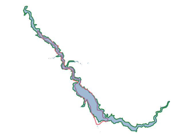

Here the green outline shows the adjusted polygon, the red outline shows the original polygon, and the background blue shows the water bodies data from the CCI.

Pour points

Pour points are the locations where rivers pour into and out of reservoirs. For many reservoirs, pour points can be found automatically. The pour in point(s) – where the upstream river(s) join reservoirs – typically experience the largest difference in accumulated flow, which can be computed directly from FAC hydrology data. The pour out point – the dam location – is often known. This can also be derived using the maximum FAC value of the reservoir. For other reservoirs, pour points need to be determined by users and in our package we have developed a Shiny app which lets users select pour points using a leaflet map. This is for reservoirs with irregular shapes or when many rivers feed into a single reservoir.

# automatically get pour points using reservoir and flow accumulation data 
pourpoints <- autogetpourpoints(
    reservoir = tehri_adjusted, 
    fac = tehri_fac_utm)
st_crs(pourpoints) <- st_crs(tehri_adjusted) 

# convert flow accumulation data to a data frame for plotting

facdf <- as.data.frame(tehri_fac_utm, xy = T)

ggplot() +
  geom_tile(data = facdf, aes(x = x, y = y)) +
  geom_sf(data = tehri_adjusted) +
  geom_sf(data = pourpoints, aes(col = as.factor(direction))) +
  scale_color_manual(
    values = c('#228833','#EE6677'),
    labels = c("Pour in", "Pour out")) +
  theme_void() +
  labs(col = "")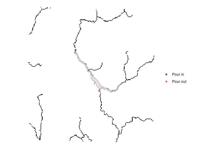

Build river lines

To map river paths digitally, we built an algorithm using Digital Elevation Model (DEM) data and Flow ACumulation data (FAC). We recommend using HydroSHEDS 15s data as input data for the algorithm. The DEM contains the average elevation in each grid cell in meters. FAC values are unitless, and simply measure the aggregated number of cells (in this case ~450m grid cells) that have accumulated to form the river at each cell. If a river was 200 cells long, and was joined by another 300 cells long, the flow accumulation one cell downstream of the confluence would be 501.

For the downstream river line the algorithm begins at the point in the reservoir with the highest accumulation. It searches nearby grid cells in the FAC data which are ‘water’ and selects the nearest point with a higher accumulation and a lower elevation. This is an iterative process, and continues for as far downstream as the user wishes to consider. For us, the default is 100km downstream.

For the upstream river line the algorithm begins at the point in the reservoir with the lowest accumulation. It searches nearby points which have water of a similar accumulation (to eliminate the river being diverted to insignificant upstream springs). Of these cells, it selects the nearest point with a lower accumulation and a higher elevation. This process is again repeated iteratively up to a set distance away from the reservoir.

riverpoints <- lapply(X = 1:2, # for each of the two pourpoints
                      FUN = getriverpoints, # run the getriverpoints function
                      reservoir = tehri_adjusted, 
                      pourpoints = pourpoints,
                      river_distance = 30000,
                      ac_tolerance = 50,
                      e_tolerance = 10, 
                       nn = 20, 
                      fac = tehri_fac_utm,
                      dem = tehri_dem_utm)

# converts each list of points into an sf LINESTRING

riverlines <- pointstolines(riverpoints, espg = espg)

ggplot(tehri_adjusted) +
  geom_sf() +
  geom_sf(data = riverlines[[1]], col = '#EE6677') +
  geom_sf(data = riverlines[[2]], col = '#4477AA') +
  theme_void()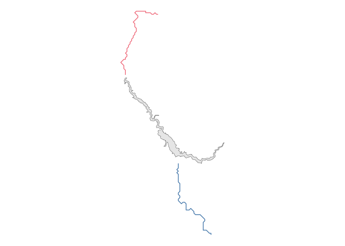

This is done with the riverpoints function. The river_distance parameter sets how far upstream and downstream to follow the river. The nn parameter sets the number of nearest neighbours (water bodies) to assess for these conditions. The ac_tolerance parameter sets a threshold for the point-to-point flow accumulation increase. This is so that at major confluences the algorithm will stop finding points downstream. The e_tolerance parameter sets a threshold for the acceptable elevation increase if there are no points downstream (upstream) which have a lower (higher) elevation. This is important as downstream points can erroneously have a slightly higher elevation value in steep gorges because DEM values are an average across an area which can be larger than the width of rivers.

The pointstolines function converts the points and associated information generated by riverpoints to an sf linestring.

Build AOI polygons

# creates buffers around river lines and reservoir buffers.

bnb <- basinandbuffers(
  reservoir = tehri_adjusted,
  upstream = riverlines[[1]],
  downstream = riverlines[[2]],
  basins = basins_tehri_utm,
  streambuffersize = 1500,
  reservoirbuffersize = 3000)

ggplot(bnb[[1]] %>% mutate(area = c("res", "down", "up"))) +
  geom_sf(aes(fill = as.factor(area)), alpha = 0.3) +
  geom_sf(data = bnb[[2]] %>% mutate(area = c("res", "down", "up")),
          aes(fill = as.factor(area))) +
  geom_sf(data = tehri_adjusted, fill = "grey") +
  theme_void()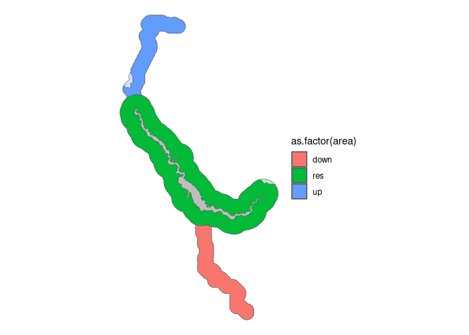

The basinsandbuffers function extracts buffers for the lines and reservoir first. The streambuffersize parameter defines the size of the buffer around river lines. The reservoirbuffersize parameter defines the size of buffer around the reservoir. Once buffers have been calculated, the function clips these areas by the river basins, so that areas beyond topographical barriers to water are not considered. Here shows the overlay of clipped polygons and the buffers themselves in lighter tone.

Dam systems

Some rivers have many connected dams and reservoirs. The method we propose for such dam systems is to first calculate AOIs for each dam in the system and second to correct these polygons to avoid overlapping areas. The makesystems function implements this using the AOIs for all dams which form a system on the same river. Reservoirs for each dam are combined into an sf MULTIPOLYGON of all reservoirs. Areas around reservoirs are combined, ensuring that they exclude any areas which are reservoirs of other dams on the system. Upstream areas are defined as the upstream area of the reservoir in the system with the highest elevation. Downstream areas are defined as the downstream area of the reservoir in the system with the lowest elevation. And “between” areas include any rivers which flow between reservoirs, which are not captured in the areas around reservoirs. The bwru parameter controls whether to crop any “between” areas to the bounding box of the all system reservoir polygons. The betweenthreshold parameter sets the minimum area for an AOI polygon to be included (default 1km²) to avoid AOIs with many small geometries.

# gets names of reservoirs to be combined into the same system

system <- damAOI::system %>% st_set_crs(3857)
names <- unique(system$name)

system_corrected <- makesystem(
  names = names, 
  aois = system)

ggplot() +
  geom_sf(data = system_corrected, aes(fill = area))  +
  theme_void() +
  labs(fill = "")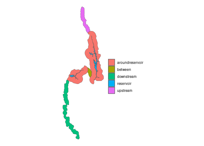

Three optional parameters to the makesystems function allow for custom overriding of the default settings. By default, the system will be named after the dam in the system with the highest elevation. This can be set manually with the systemname parameter, for example if a large reservoir exists between two smaller reservoirs. The defaults as to the reservoirs for which the upstream and downstream areas of the system are taken from can also be set manually with the uprivers and downrivers parameters. This is useful when, for example, the rivers downstream of two dams meet at a confluence, with a third reservoir further downriver. In such a case, users may want to consider the upriver segments of both reservoirs as part of the Area of Interest.

These binaries (installable software) and packages are in development.
They may not be fully stable and should be used with caution. We make no claims about them.