The hardware and bandwidth for this mirror is donated by METANET, the Webhosting and Full Service-Cloud Provider.
If you wish to report a bug, or if you are interested in having us mirror your free-software or open-source project, please feel free to contact us at mirror[@]metanet.ch.

diegr

Overview

The name diegr comes from Dynamic and Interactive EEG Graphics using R. The diegr package enables researchers to visualize high-density electroencephalography (HD-EEG) data with animated and interactive graphics, supporting both exploratory and confirmatory analyses of sensor-level brain signals.

The package diegr includes:

• interactive boxplots (boxplot_epoch, boxplot_subject, boxplot_rt)
• interactive waveforms (interactive_waveforms)
• topographic maps in 2D (topo_plot)
• scalp plots in 3D (scalp_plot)
• functions for computing summary statistics, baseline correction, pointwise and jackknife mean (summary_stats_rt,baseline_correction, compute_mean)
• functions for easy selection of subdata or region of interest (pick_data, pick_region)
• functions for plotting the mean with pointwise confidence interval (plot_time_mean, plot_topo_mean)
• animations of time course of the raw signal or the average in 2D and 3D (animate_topo, animate_topo_mean, animate_scalp)

Installation

You can install the current version of diegr from CRAN with:

install.packages("diegr")

or the latest development version from GitHub with:

# install.packages("devtools")
devtools::install_github("gerslovaz/diegr") 

Data

Because of large volumes of data obtained from HD-EEG measurements, the package allows users to work directly with database tables (in addition to common formats such as data frames or tibbles). Such a procedure is more efficient in terms of memory usage.

The database you want to use as input to diegr functions must contain columns with the following structure:

• group - ID of groups,
• subject - ID of subjects,
• sensor - sensor labels,
• epoch - epoch numbers,
• condition - labels of experimental condition,
• time - numbers of time points (as sampling points, not in ms),
• signal - the EEG signal amplitude in microvolts (in most functions it is possible to set the name of the column containing the amplitude arbitrarily).

Note: It is not necessary for the data to contain all variables, but if it does, they must be named according to the structure presented above.

The package contains some included training datasets:

• epochdata: epoched HD-EEG data (anonymized short slice from big HD-EEG study presented in Madetko-Alster, 2025) for 2 subjects and 204 selected sensors in 50 time points,
• HCGSN256: a list with Cartesian coordinates of HD-EEG sensor positions in 3D space on the scalp surface and their projection into 2D space
• rtdata: response times (time between stimulus presentation and pressing the button) from the experiment involving a simple visual motor task (anonymized short slice from big HD-EEG study presented in Madetko-Alster, 2025).

For more information about the structure of built-in data see the package vignette vignette("diegr", package = "diegr").

Quick examples

Interactive boxplot

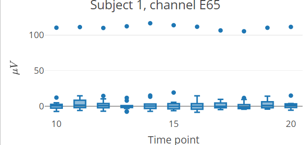
This is a basic example which shows how to plot interactive epoch boxplots from chosen electrode in different time points for one subject:

library(diegr)
data("epochdata")

epochdata |>
  pick_data(subject_rg = 1, sensor_rg = "E65") |>
boxplot_epoch(amplitude = "signal", time_lim = c(10:20))

Note: The README format does not allow the inclusion of plotly interactive elements, only the static preview of the result is shown.

Topographic map

data("HCGSN256")
# creating a mesh
M1 <- point_mesh(dimension = 2, n = 30000, type = "polygon", sensor_select = unique(epochdata$sensor))
# filtering a subset of data to display 
data_short <- epochdata |>
  pick_data(subject_rg = 1, time_rg = 15, epoch_rg = 10)
# or you can use dplyr::filter()
# dplyr::filter(subject == 1 & epoch == 10 & time == 15) 
# function for displaying a topographic map of the chosen signal on the created mesh M1
topo_plot(data_short, amplitude = "signal", mesh = M1)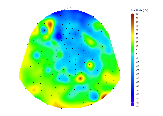

Computing and displaying the average in time domain

Compute the average signal for subject 2 from the channels E65 and E34 (exclude the oulier epochs 14 and 15) and then display it along with CI bounds (use plot_time_mean conditioned by sensor)

# extract required data
edata <- epochdata |>
  pick_data(subject_rg = 2, sensor_rg = c("E34", "E65"), epoch_rg = 1:13)
# baseline correction
data_base <- baseline_correction(edata, baseline_range = 1:10)
# compute average
data_mean <- data_base |> 
  compute_mean(amplitude = "signal_base", type = "point", domain = "time")
# plot the average line with CI
plot_time_mean(data = data_mean, t0 = 10, condition_column = "sensor", legend_title = "Sensor")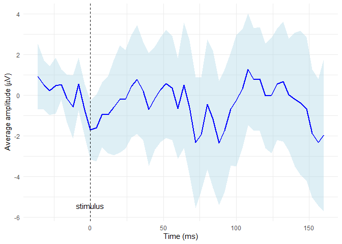

For detailed examples and usage explanation, please see the package vignette: vignette("diegr", package = "diegr").

References Madetko-Alster N., Alster P., Lamoš M., Šmahovská L., Boušek T., Rektor I. and Bočková M. The role of the somatosensory cortex in self-paced movement impairment in Parkinson’s disease. Clinical Neurophysiology. 2025, vol. 171, 11-17. https://doi.org/10.1016/j.clinph.2025.01.001

License This package is distributed under the MIT license. See LICENSE file for details.

Citation Use citation("diegr") to cite this package.

These binaries (installable software) and packages are in development.
They may not be fully stable and should be used with caution. We make no claims about them.