The hardware and bandwidth for this mirror is donated by METANET, the Webhosting and Full Service-Cloud Provider.
If you wish to report a bug, or if you are interested in having us mirror your free-software or open-source project, please feel free to contact us at mirror[@]metanet.ch.

Divvy up diversity into geographic regions of fair comparison!
An R package offering spatial subsampling functions for biogeography and biodiversity studies, whether analysing fossil or modern taxon occurrence data, as described by: Antell, G.T., Benson, R.B., and Saupe, E.E. (2024). Spatial standardization of taxon occurrence data—a call to action. Paleobiology, 50(2), 177-193. https://doi.org/10.1017/pab.2023.36.
Three types of subsampling are available to to standardise the number and maximum spread (dispersion) of sites within a region of specified size:
cookies: Imposes a radial constraint on the spatial
bounds of a subsample and standardises area by rarefying the number of
localities
clustr: Aggregates sites that are nearest neighbours
(connecting them with a minimum spanning tree) to impose a maximum
diameter on the spatial bounds of a subsample, and optionally rarefies
localities
bandit: Rarefies the number of localities within
bands of equal latitude
Additional functions include uniqify to subset an
occurrence dataset to unique taxon-coordinate combinations,
sdSumry to calculate basic spatial coverage and diversity
metadata for a dataset or its subsamples, rangeSize to
calculate five measures of geographic range size, and
classRast to generate a raster containing the most common
environment or trait for point occurrences falling in each grid
cell.
There are vignettes accompanying the package, to demonstrate use
cases of divvy functions and describe common considerations
for analyses of taxonomic occurrence data. You can view the compiled
documents at the package
website under ‘Getting
started’.
You can install the newest release of divvy from
CRAN:
install.packages('divvy')Alternatively, you can install the development version of
divvy from GitHub with
help from devtools:
# install.packages('devtools')
devtools::install_github('GawainAntell/divvy')bivalves: Package data(Palaeo)ecologists often want to inspect basic information about
taxon occurrence datasets such as number of occurrences, number of
unique localities, general size and position of the study region, and
biodiversity. This may be an initial step to become acquainted with the
data, or it may be a final step of analysis to estimate ecological
variables of interest. Let’s load one of the example datasets in with
divvy to demonstrate some functions that may help analyse
it. The occurrences are latitude-longitude point coordinates of Pliocene
bivalves from the Paleobiology Database; before proceeding further,
let’s rasterise these into an equal-area grid, a common starting point
for biogeography analysis.
library(divvy)
data('bivalves')

# initialise Equal Earth projected coordinates
library(terra)
rWorld <- rast()
prj <- 'EPSG:8857'
rPrj <- project(rWorld, prj, res = 200000) # 200,000m is approximately 2 degrees
values(rPrj) <- 1:ncell(rPrj)

# coordinate column names for the current and target coordinate reference system
xyCartes <- c('paleolng','paleolat')
xyCell   <- c('cellX','cellY')

# extract cell number and centroid coordinates associated with each occurrence
llOccs <- vect(bivalves, geom = xyCartes, crs = 'epsg:4326')
prjOccs <- project(llOccs, prj)
bivalves$cell <- cells(rPrj, prjOccs)[,'cell']
bivalves[, xyCell] <- xyFromCell(rPrj, bivalves$cell)uniqify:
Subset to unique occurrencesNow let’s examine the data with some divvy functions.
First, we can apply uniqify to leave out any duplicate
occurrences of a taxon within a grid cell. This shortens the dataset
(and thereby reduces memory use) by more than half.
nrow(bivalves)
#> [1] 8095
bivalves <- uniqify(bivalves, taxVar = 'genus', xy = xyCell)
nrow(bivalves)
#> [1] 3061sdSumry:
Summary spatial and diversity metricsHow many taxa are there? Over how many sites (equal-area grid cells)?
How many degrees of latitude do those sites span? The
sdSumry function returns this and related spatial and
diversity metadata.
sdSumry(bivalves, taxVar = 'genus', xy = xyCell, crs = prj)
#>      nOcc nLoc centroidX centroidY latRange greatCircDist meanPairDist
#> [1,] 3061  157 -434404.9   1647720 137.4159      28917.12     11375.07
#>      minSpanTree     SCOR nTax
#> [1,]    93349.91 20.64401  550
There are just over 3000 unique taxon-site occurrences, including 550 genera from 157 grid cells across 137 degrees latitude.
rangeSize:
Calculate geographic range sizeMaybe we aren’t interested in community ecology and instead care
about the geographic distribution of focal taxa, such as the mussel
Mytilus and scallop Yabepecten. Provide the
coordinates for these two taxa to divvy’s
rangeSize function:
myti <- bivalves[bivalves$genus == 'Mytilus',    xyCell]
yabe <- bivalves[bivalves$genus == 'Yabepecten', xyCell]

rangeSize(myti, crs = prj)
#>      nLoc centroidX centroidY latRange greatCircDist meanPairDist minSpanTree
#> [1,]   18  67152.05   4750551 99.31458      22351.73     10390.96    37303.68
rangeSize(yabe, crs = prj)
#>      nLoc centroidX centroidY latRange greatCircDist meanPairDist minSpanTree
#> [1,]    2  11856041   5039440 1.808585           200          200         200
Mytilus is observed in 18 grid cells spread over tens of thousands of kilometers. In contrast, Yabepecten occurs in only two localities, 200 km apart at their grid cell centroids.
If we back-transform the two locality’s coordinates from Equal Earth projection to familiar latitude-longitude, we can tell Yabepecten has been reported only in northern Honshu, Japan (140-141 E longitude, 40-42 N latitude).
yabeVect <- vect(yabe, geom = xyCell, crs = prj)
project(yabeVect, 'epsg:4326')
#>  class       : SpatVector
#>  geometry    : points
#>  dimensions  : 2, 0  (geometries, attributes)
#>  extent      : 139.6679, 141.3001, 40.16519, 41.97377  (xmin, xmax, ymin, ymax)
#> coord. ref. : lon/lat WGS 84 (EPSG:4326)cookies:
Subsample global data into equivalent regionsThe bivalves dataset spans most of the world’s oceans.
If we were interested in a question such as how diversity at this
Pliocene time step compares against diversity from an earlier interval
when geographic sampling coverage was much more limited, we’d have to
account for this different data distribution—otherwise, we’d unfairly
estimate the well-sampled Pliocene to be far more diverse. Geographic
standardisation of both area (acreage or number of sites studied) and
dispersion (amount sites are spread apart) allows fair comparisons of
ecological variables like richness, whether between time steps,
environments, or other comparison groups with heterogeneous spatial
coverage.
divvy offers three functions for subsampling
(cookies, clustr, and bandit)
which differ in how they standardise for dispersion. The easiest form of
subsampling to visualise is applying a circular constraint to define the
bounds of a subsample region. Within that region, a given number of
sites are selected, to standardise area. Here, let’s take 10 subsamples
of the bivalves occurrences, each containing 12 sites
within a circular region of 1500km (about the size of Australia.)
set.seed(1)
circLocs <- cookies(dat = bivalves, xy = xyCell,
                    iter = 10, nSite = 12, r = 1500,
                    crs = prj, output = 'full')
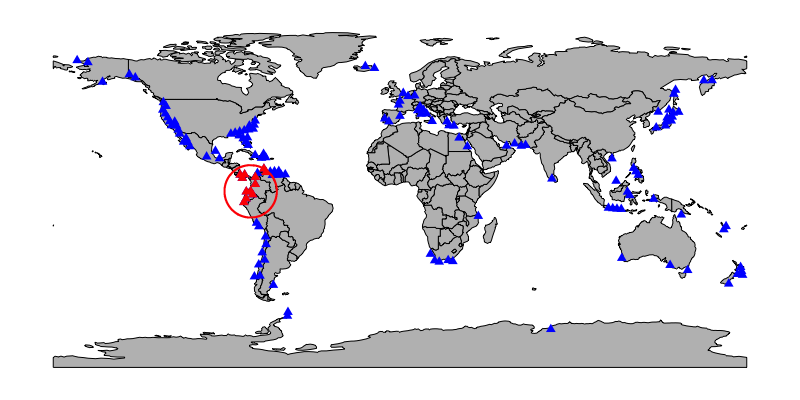
Below is a map of one possible subsample (red, with regional constraint drawn around it). Sites not included in the subsample, including one within the regional constraint, are plotted in blue.

An individual subsample (one data.frame element of the
returned list object) contains all occurrences from the
subsampled sites. Here’s a peek at the first subsample, to show it’s
just a subset of bivalves.
str(circLocs[[1]])
#> 'data.frame':    338 obs. of  12 variables:
#>  $ genus        : chr  "Anomia" "Chlamys" "Mercenaria" "Ostrea" ...
#>  $ paleolng     : num  -80.5 -80.5 -80.5 -80.5 -87.4 ...
#>  $ paleolat     : num  27.5 27.5 27.5 27.5 31 ...
#>  $ collection_no: int  41496 41496 41496 41496 41824 58893 58893 58893 58893 58893 ...
#>  $ reference_no : int  11119 11119 11119 11119 11118 16700 16700 16700 16700 16700 ...
#>  $ environment  : chr  "marine indet." "marine indet." "marine indet." "marine indet." ...
#>  $ max_ma       : num  5.33 5.33 5.33 5.33 5.33 ...
#>  $ min_ma       : num  3.6 3.6 3.6 3.6 3.6 ...
#>  $ accepted_name: chr  "Anomia simplex" "Chlamys" "Mercenaria campechiensis" "Ostrea" ...
#>  $ cell         : num  4178 4178 4178 4178 3832 ...
#>  $ cellX        : num  -7343959 -7343959 -7343959 -7343959 -7743959 ...
#>  $ cellY        : num  3539440 3539440 3539440 3539440 3939440 ...
Because each subsample has the same information structure as the
original dataset, we can analogously calculate summary spatial and
diversity data for them using sdSumry. Each row of the
returned matrix corresponds to one of the ten subsamples. In this small
group of replicate subsamples, regional richness ranges from 117 to 194
genera. The number of localities is always 12, as was specified above,
and the dispersion of subsamples is always within the upper bound set by
the diameter of 3,000km (e.g. maximum great circle distance across any
subsample’s sites is 2807km).
sdSumry(circLocs, taxVar = 'genus', xy = xyCell, crs = prj)
#>    nOcc nLoc   centroidX centroidY latRange greatCircDist meanPairDist
#> 1   338   12  -6977292.4   4156106 10.25901      1612.452     781.6607
#> 2   265   12 -10160625.7   4072773 17.14477      2039.608     910.6453
#> 3   410   12  -6727292.4   2356106 17.67042      2720.294    1289.9956
#> 4   252   12 -10127292.4   3889440 18.77490      2209.072     888.0877
#> 5   460   12  -6993959.1   4056106 11.91278      1720.465     757.5157
#> 6   446   12    406040.9   5589440 11.37344      1562.050     833.9107
#> 7   293   12 -10177292.4   4239440 20.61302      2408.319     866.7620
#> 8   224   12 -10127292.4   5239440 27.00700      2807.134    1119.3347
#> 9   446   12    406040.9   5589440 11.37344      1562.050     833.9107
#> 10  350   12    256040.9   5389440 14.91345      1811.077    1047.1642
#>    minSpanTree     SCOR nTax
#> 1     2814.214 33.87300  141
#> 2     2800.000 26.46397  121
#> 3     4097.770 40.52424  194
#> 4     2847.214 25.14927  117
#> 5     2731.371 48.65573  166
#> 6     3402.094 44.22359  190
#> 7     2965.685 29.02605  130
#> 8     3665.081 21.11620  121
#> 9     3402.094 44.22359  190
#> 10    4287.575 33.92261  163
These binaries (installable software) and packages are in development.
They may not be fully stable and should be used with caution. We make no claims about them.