 Now we construct a sequence of tuning parameters with length K = 10.
The hardware and bandwidth for this mirror is donated by METANET, the Webhosting and Full Service-Cloud Provider.
If you wish to report a bug, or if you are interested in having us mirror your free-software or open-source project, please feel free to contact us at mirror[@]metanet.ch.
dpcc aims to enable fast computation and path
visualization of L1 convex clustering with identical weights.
You can install dpcc from GitHub with:
# install.packages("dpcc")
devtools::install_github("bingyuan-zhang/dpcc")
Load the packages.
library(dpcc)We first generate the three clusters example.
#install.packages("ggplot2")
library(ggplot2)
set.seed(12)
n = 50
error = matrix(rnorm(n*2,sd = 1.4),n,2)
which=sample(1:3, n, replace=TRUE)
xmean = matrix(rnorm(3*2,sd = 11),3,2)
tb1 = error + xmean[which,]
data = data.frame(
  x = scale(tb1[,1]),
  y = scale(tb1[,2]),
  clusters = factor(which)
)

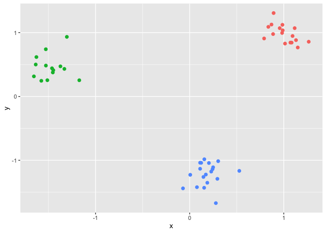
ggplot(data,aes(x,y,color=factor(clusters))) +
  geom_point(size = 2, show.legend = FALSE)
Now we construct a sequence of tuning parameters with length K = 10.
dat = data.matrix(data)[,1:2]
lam_max = find_lambda(dat)/1.5;
K = 10
Lam = sapply(1:K, function(i) i/K*lam_max)

Lam
#>  [1] 0.002726164 0.005452327 0.008178491 0.010904655 0.013630819 0.016356982
#>  [7] 0.019083146 0.021809310 0.024535474 0.027261637
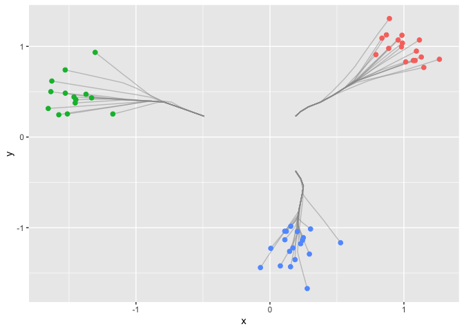
Next we use the function in the package to draw the clusterpath.
res = cpaint(dat,Lam)
df.paths <- data.frame(x = dat[,1],y = dat[,2], group=1:n)
for (j in 1:K) {
  df <- data.frame(x=res[[1]][j,], y=res[[2]][j,], group=1:n)
  df.paths <- rbind(df.paths,df)
}

ggplot(data) +
  geom_path(data = df.paths, aes(x = x, y = y, group=group), colour='grey60', alpha = 0.5) +
  geom_point(aes(x = x, y = y, col = clusters), size = 2, show.legend = FALSE)
[1.] [Dynamic visualization for L1 fusion convex clustering in near-linear time] Bingyuan Zhang, Yoshikazu Terada, Jie Chen (UAI 2021 to appear).
These binaries (installable software) and packages are in development.
They may not be fully stable and should be used with caution. We make no claims about them.