
The hardware and bandwidth for this mirror is donated by METANET, the Webhosting and Full Service-Cloud Provider.
If you wish to report a bug, or if you are interested in having us mirror your free-software or open-source project, please feel free to contact us at mirror[@]metanet.ch.
The goal of ecotrends is to compute a time
series of ecological niche models, using species occurrence
data and environmental variables, and then map the existence and
direction of linear temporal trends in environmental
suitability, as in Arenas-Castro
& Sillero (2021).
This package is part of the MontObEO project.
Here is a very basic flow chart of the package:
You can (re)install ecotrends from GitHub and then load
it:
# devtools::install_github("AMBarbosa/ecotrends")  # run if you don't have the latest version!

library(ecotrends)You’ll need some species presence coordinates. The code below downloads some example occurrence data from GBIF (just from a couple of years, to avoid the example taking a long time to download), and then performs just a basic automatic cleaning:
library(geodata)
#> Loading required package: terra
#> terra 1.8.54
library(fuzzySim)

occ_raw <- geodata::sp_occurrence(genus = "Chioglossa",
                                  species = "lusitanica",
                                  args = c("year=2022,2024"),
                                  fixnames = FALSE)
#> Loading required namespace: jsonlite
#> 509 records found
#> 0-300-509
#> 509 records downloaded

occ_clean <- fuzzySim::cleanCoords(data = occ_raw,
                                   coord.cols = c("decimalLongitude", "decimalLatitude"),
                                   uncert.col = "coordinateUncertaintyInMeters",
                                   uncert.limit = 10000,
                                   abs.col = "occurrenceStatus",
                                   plot = FALSE)
#> 509 rows in input data
#> 477 rows after 'rm.dup'
#> 477 rows after 'rm.equal'
#> 477 rows after 'rm.imposs'
#> 477 rows after 'rm.missing.any'
#> 477 rows after 'rm.zero.any'
#> 476 rows after 'rm.imprec.any'
#> 33 rows after 'rm.uncert' (with uncert.limit=10000 and uncert.na.pass=TRUE)
#> 33 rows after 'rm.abs'

occ_coords <- occ_clean[ , c("decimalLongitude", "decimalLatitude")]You should also delimit a region for modelling. You can provide your own spatial extent or polygon – e.g., a biogeographical region that is within your species’ reach, and within which that species was reasonably surveyed (mind that pixels within your region that don’t overlap species presences are taken by Maxent as available and unoccupied). Alternatively or additionally, you can use e.g. the code below to compute a reasonably sized area around your species occurrences (see help file and try out different options, some of which may be much more adequate for your particular case!):
reg <- fuzzySim::getRegion(pres.coords = occ_coords,
                           CRS = "EPSG:4326",  # make sure it's correct for your data!
                           type = "width",
                           width_mult = 0.5,
                           dist_mult = 1)

countries <- geodata::world(path = "outputs/countries")

plot(countries, add = TRUE)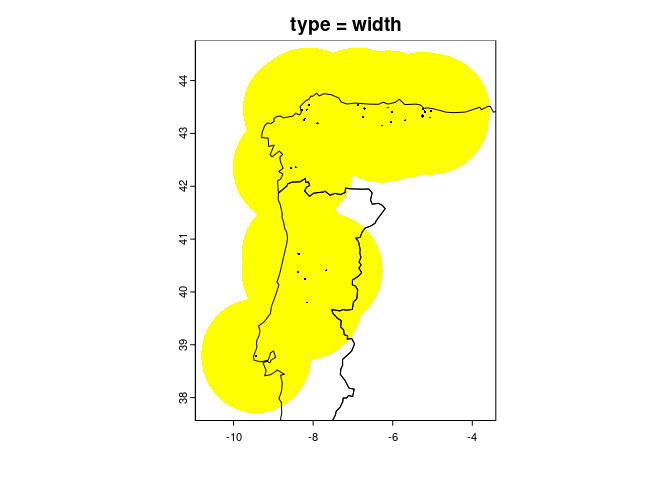
Now let’s download some variables with which to
build a yearly time series of ecological niche models
for this species in this region. You can first use the
varsAvailable function to check which variables and years
are available through the ecotrends package, and then the
getVariables function to download the ones you choose
(unless you want to use your own variables from elsewhere). Mind that
the download may take a long time:
ecotrends::varsAvailable()
#> $TerraClimate
#> $TerraClimate$vars
#>  [1] "ws"   "vpd"  "vap"  "tmin" "tmax" "swe"  "srad" "soil" "g"    "ppt"
#> [11] "pet"  "def"  "aet"  "PDSI"
#>
#> $TerraClimate$years
#>  [1] 1958 1959 1960 1961 1962 1963 1964 1965 1966 1967 1968 1969 1970 1971 1972
#> [16] 1973 1974 1975 1976 1977 1978 1979 1980 1981 1982 1983 1984 1985 1986 1987
#> [31] 1988 1989 1990 1991 1992 1993 1994 1995 1996 1997 1998 1999 2000 2001 2002
#> [46] 2003 2004 2005 2006 2007 2008 2009 2010 2011 2012 2013 2014 2015 2016 2017
#> [61] 2018 2019 2020

vars <- ecotrends::getVariables(vars = c("tmin", "tmax", "ppt", "pet", "ws"),
                                years = 1981:1990,
                                region = reg,
                                file = "outputs/variables")
#> Variables imported from the specified 'file', which already exists in the current working directory. Please provide a different 'file' path/name if this is not what you want.

names(vars)
#>  [1] "tmin_1981" "tmin_1982" "tmin_1983" "tmin_1984" "tmin_1985" "tmin_1986"
#>  [7] "tmin_1987" "tmin_1988" "tmin_1989" "tmin_1990" "tmax_1981" "tmax_1982"
#> [13] "tmax_1983" "tmax_1984" "tmax_1985" "tmax_1986" "tmax_1987" "tmax_1988"
#> [19] "tmax_1989" "tmax_1990" "ppt_1981"  "ppt_1982"  "ppt_1983"  "ppt_1984"
#> [25] "ppt_1985"  "ppt_1986"  "ppt_1987"  "ppt_1988"  "ppt_1989"  "ppt_1990"
#> [31] "pet_1981"  "pet_1982"  "pet_1983"  "pet_1984"  "pet_1985"  "pet_1986"
#> [37] "pet_1987"  "pet_1988"  "pet_1989"  "pet_1990"  "ws_1981"   "ws_1982"
#> [43] "ws_1983"   "ws_1984"   "ws_1985"   "ws_1986"   "ws_1987"   "ws_1988"
#> [49] "ws_1989"   "ws_1990"
plot(vars[[1:6]])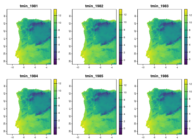
These variable raster layers have a given pixel size in geographic degrees, with a nominal pixel size at the Equator, but (as the longitude meridians all converge towards the poles) actual pixel sizes can vary widely across latitudes. So, let’s check the average pixel size in our study region, as well as the spatial uncertainty values of our occurrence coordinates:
sqrt(ecotrends::pixelArea(vars))![]()
#> Mean pixel area (m2):
#> 16321122.5160472
#> [1] 4039.941

summary(occ_clean$coordinateUncertaintyInMeters, na.rm = TRUE)
#>    Min. 1st Qu.  Median    Mean 3rd Qu.    Max.    NA's
#>    1000    1000    1000    1000    1000    1000       3
You can see there are several occurrence points with spatial uncertainty larger than our pixel size, so it might be a good idea to coarsen the spatial resolution of the variable layers:
vars_agg <- terra::aggregate(vars,
                             fact = 2)

sqrt(ecotrends::pixelArea(vars_agg))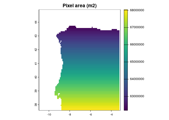
#> Mean pixel area (m2):
#> 65290574.0163304
#> [1] 8080.258
This is much closer to the spatial resolution of many of the species occurrences.
We can now compute yearly ecological niche models with these occurrences and variables, optionally saving the results to a file:
mods <- ecotrends::getModels(occs = occ_coords,
                             rasts = vars_agg,
                             region = reg,
                             nbg = 10000,
                             nreps = 3, # increase 'nreps' for more robust (albeit slower) results
                             collin = TRUE,
                             maxcor = 0.75,
                             maxvif = 5,
                             classes = "default",
                             regmult = 1,
                             file = "outputs/models")
#> Models imported from the specified 'file', which already exists in the current working directory. Please provide a different 'file' path/name if this is not what you want.
Note that (if you have fuzzySim >= 4.26 installed)
you can add a bias layer to drive the selection of
background points to incorporate survey effort, if your study area
contains more pixels than nbg. See the
?getModels help file for more details.
You can compute the permutation importance of each variable in each of the output models, as well as the mean and standard deviation across replicates for each year:
set.seed(1)  # to make next output reproducible

varimps <- ecotrends::getImportance(mods,
                                    nper = 10, # increase 'nper' for more robust (albeit slower) results
                                    plot = TRUE,
                                    main = "Mean variable importance",
                                    ylab = "",
                                    las = 2)
#> computing period 1 of 10 (with replicates): 1981
#> computing period 2 of 10 (with replicates): 1982
#> computing period 3 of 10 (with replicates): 1983
#> computing period 4 of 10 (with replicates): 1984
#> computing period 5 of 10 (with replicates): 1985
#> computing period 6 of 10 (with replicates): 1986
#> computing period 7 of 10 (with replicates): 1987
#> computing period 8 of 10 (with replicates): 1988
#> computing period 9 of 10 (with replicates): 1989
#> computing period 10 of 10 (with replicates): 1990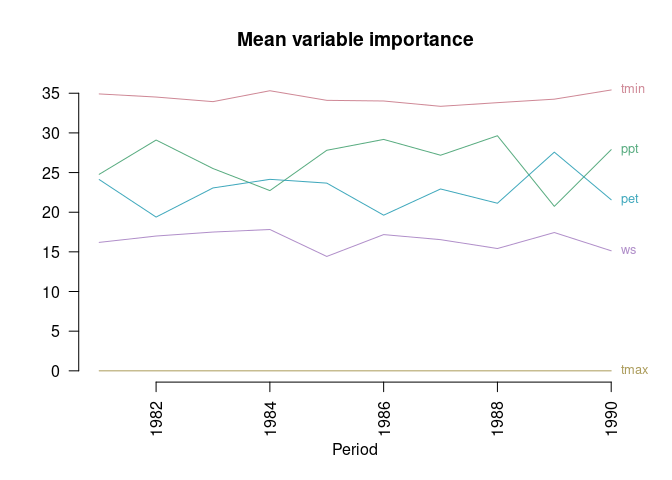
head(varimps, 8)
#>   period  variable     rep1     rep2     rep3     mean        sd
#> 1   1981 tmin_1981 34.08416 37.20650 33.44227 34.91098 1.6441948
#> 2   1981 tmax_1981  0.00000  0.00000  0.00000  0.00000 0.0000000
#> 3   1981  ppt_1981 26.97670 20.82831 26.52798 24.77766 2.7986177
#> 4   1981  pet_1981 24.07393 26.34771 21.92923 24.11695 1.8040937
#> 5   1981   ws_1981 14.86521 15.61749 18.10053 16.19441 1.3823769
#> 6   1982 tmin_1982 34.25688 33.98315 35.31589 34.51864 0.5747116
#> 7   1982 tmax_1982  0.00000  0.00000  0.00000  0.00000 0.0000000
#> 8   1982  ppt_1982 27.68860 30.90411 28.70352 29.09874 1.3421438
Note that the output plot does not reflect the deviations around the mean importance of each variable each year (see this value in the output table); and that the plot may become too crowded if there are many variables or if their importances overlap. Note also that “variable importance” is a vague concept which can be measured in several different ways, with potentially varying results!
Let’s now compute the model predictions for each year, optionally delimiting them to the modelled region (though you can predict on a larger or an entirely different region, assuming that the species-environment relationships are the same as in the modelled region), and optionally exporting the results to a file:
preds <- ecotrends::getPredictions(rasts = vars_agg,
                                   mods = mods,
                                   region = reg,
                                   type = "cloglog",
                                   clamp = TRUE,
                                   file = "outputs/predictions")
#> Predictions imported from the specified 'file', which already exists in the current working directory. Please provide a different 'file' path/name if this is not what you want.

names(preds)
#>  [1] "1981" "1982" "1983" "1984" "1985" "1986" "1987" "1988" "1989" "1990"
plot(preds[[1]], range = c(0, 1), nr = 1)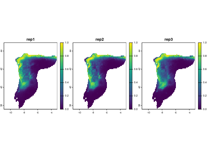
You can also map the mean prediction across replicates per year:
preds_mean <- terra::rast(lapply(preds, terra::app, "mean"))
plot(preds_mean, nr = 2)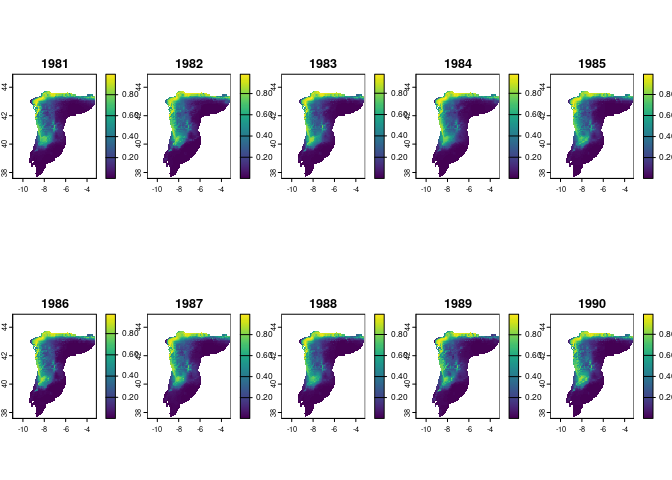
You can evaluate the fit of these predictions to the model training data:
par(mfrow = c(2, 2))

perf <- ecotrends::getPerformance(rasts = preds,
                                  mods = mods,
                                  plot = FALSE)
#> evaluating period 1 of 10 (with replicates): 1981
#> evaluating period 2 of 10 (with replicates): 1982
#> evaluating period 3 of 10 (with replicates): 1983
#> evaluating period 4 of 10 (with replicates): 1984
#> evaluating period 5 of 10 (with replicates): 1985
#> evaluating period 6 of 10 (with replicates): 1986
#> evaluating period 7 of 10 (with replicates): 1987
#> evaluating period 8 of 10 (with replicates): 1988
#> evaluating period 9 of 10 (with replicates): 1989
#> evaluating period 10 of 10 (with replicates): 1990

head(perf)
#>   period rep train_presences test_presences train_AUC  test_AUC train_TSS
#> 1   1981   1             110             28 0.8740956 0.8518081 0.6558619
#> 2   1981   2             110             28 0.8672644 0.8878075 0.6124322
#> 3   1981   3             110             28 0.8729622 0.8618532 0.6273246
#> 4   1982   1             110             28 0.8819149 0.8482923 0.6715075
#> 5   1982   2             110             28 0.8690163 0.8959793 0.6228879
#> 6   1982   3             110             28 0.8777651 0.8681924 0.6317854
#>   train_thresh_TSS  test_TSS test_thresh_TSS train_kappa train_thresh_kappa
#> 1             0.38 0.5808085            0.34   0.2139232               0.67
#> 2             0.41 0.7145572            0.34   0.2245709               0.64
#> 3             0.29 0.6625129            0.36   0.2201877               0.66
#> 4             0.41 0.5477819            0.43   0.2358166               0.71
#> 5             0.40 0.7404165            0.49   0.2153542               0.64
#> 6             0.47 0.6586985            0.35   0.2369446               0.82
#>   test_kappa test_thresh_kappa
#> 1 0.10641284              0.89
#> 2 0.16274823              0.99
#> 3 0.10803384              0.93
#> 4 0.11225416              0.84
#> 5 0.11627452              0.92
#> 6 0.07821233              0.89
Note that rasts here can be either the output of
getPredictions(), or a file argument
previously provided to getPredictions(), in case you
exported predictions in a previous R session and don’t want to compute
them again.
Finally, you can use the getTrend function to
get the slope and significance of a linear (monotonic) temporal
trend in suitability in each pixel (as long as there are enough
time steps with suitability values), optionally providing your
occurrence coordinates if you want the results to be restricted to the
pixels that overlap them:
trend <- ecotrends::getTrend(rasts = preds,
                             occs = occ_coords,
                             full = TRUE,
                             file = "outputs/trend")
#> Trend raster(s) imported from the specified 'file', which already exists in the current working directory. Please provide a different 'file' path/name if this is not what you want.

plot(trend,
     col = hcl.colors(100, "spectral"),
     type = "continuous")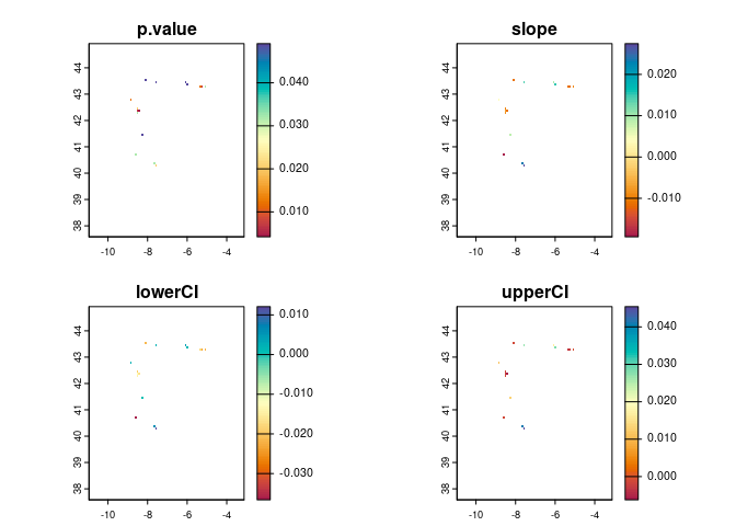
See ?trend::sens.slope to know more about these
statistics. If you want to compute only the slope layer (with only the
significant values under ‘alpha’), set full = FALSE above.
Or you can compute the full result as above, but plot just a layer
you’re interested in, and optionally add the region polygon:
plot(trend[["slope"]],
     col = hcl.colors(100, "spectral"))

plot(reg, lwd = 0.5, add = TRUE)
plot(countries, lwd = 0.8, add = TRUE)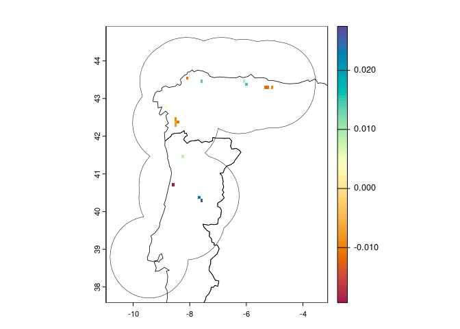
Positive slope values indicate increasing suitability, while negative
values indicate decreasing suitability over time. Pixels with no value
have no significant linear trend (or no occurrence points, if
occs are provided).
These binaries (installable software) and packages are in development.
They may not be fully stable and should be used with caution. We make no claims about them.