
The hardware and bandwidth for this mirror is donated by METANET, the Webhosting and Full Service-Cloud Provider.
If you wish to report a bug, or if you are interested in having us mirror your free-software or open-source project, please feel free to contact us at mirror[@]metanet.ch.

This R package is a wrapper of the C++ library epiworld. It provides a general framework for modeling disease transmission using agent-based models. Some of the main features include:
From the package’s description:
A flexible framework for Agent-Based Models (ABM), the epiworldR package provides methods for prototyping disease outbreaks and transmission models using a C++ backend, making it very fast. It supports multiple epidemiological models, including the Susceptible-Infected-Susceptible (SIS), Susceptible-Infected-Removed (SIR), Susceptible-Exposed-Infected-Removed (SEIR), and others, involving arbitrary mitigation policies and multiple-disease models. Users can specify infectiousness/susceptibility rates as a function of agents’ features, providing great complexity for the model dynamics. Furthermore, epiworldR is ideal for simulation studies featuring large populations.
Current available models:
Note: Measles-specific models have been moved to the
separate measles R
package.
Note: Measles-specific models have been moved to the
separate measles R
package.
ModelDiagramModelDiffNetModelSEIRModelSEIRCONNModelSEIRDModelSEIRDCONNModelSEIRMixingModelSEIRMixingQuarantineModelSIRModelSIRCONNModelSIRDModelSIRDCONNModelSIRLogitModelSIRMixingModelSISModelSISDModelSURVYou can install the development version of epiworldR from GitHub with:
devtools::install_github("UofUEpiBio/epiworldR")Or from R-universe (recommended for the latest development version):
install.packages(
  'epiworldR',
  repos = c(
    'https://uofuepibio.r-universe.dev',
    'https://cloud.r-project.org'
  )
)
Or from CRAN
install.packages("epiworldR")This R package includes several popular epidemiological models, including SIS, SIR, and SEIR using either a fully connected graph (similar to a compartmental model) or a user-defined network.
This Susceptible-Infected-Recovered model features a population of 100,000 agents simulated in a small-world network. Each agent is connected to ten other agents. One percent of the population has the virus, with a 70% chance of transmission. Infected individuals recover at a 0.3 rate:
library(epiworldR)
#> Thank you for using epiworldR! Please consider citing it in your work.
#> You can find the citation information by running
#>   citation("epiworldR")

# Creating a SIR model
sir <- ModelSIR(
  name              = "COVID-19",
  prevalence        = .01,
  transmission_rate = .7,
  recovery          = .3
) |>
  # Adding a Small world population
  agents_smallworld(n = 100000, k = 10, d = FALSE, p = .01) |>
  # Running the model for 50 days
  run(ndays = 50, seed = 1912)
#> _________________________________________________________________________
#> |Running the model...
#> |||||||||||||||||||||||||||||||||||||||||||||||||||||||||||||||||||||||| done.
#> |

sir
#> ________________________________________________________________________________
#> Susceptible-Infected-Recovered (SIR)
#> It features 100000 agents, 1 virus(es), and 0 tool(s).
#> The model has 3 states.
#> The final distribution is: 0 Susceptible, 0 Infected, and 100000 Recovered.
Visualizing the outputs
summary(sir)
#> ________________________________________________________________________________
#> ________________________________________________________________________________
#> SIMULATION STUDY
#>
#> Name of the model   : Susceptible-Infected-Recovered (SIR)
#> Population size     : 100000
#> Agents' data        : (none)
#> Number of entities  : 0
#> Days (duration)     : 50 (of 50)
#> Number of viruses   : 1
#> Last run elapsed t  : 143.00ms
#> Last run speed      : 34.82 million agents x day / second
#> Rewiring            : off
#>
#> Global events:
#>  (none)
#>
#> Virus(es):
#>  - COVID-19
#>
#> Tool(s):
#>  (none)
#>
#> Model parameters:
#>  - Recovery rate     : 0.3000
#>  - Transmission rate : 0.7000
#>
#> Distribution of the population at time 50:
#>   - (0) Susceptible :  99000 -> 0
#>   - (1) Infected    :   1000 -> 0
#>   - (2) Recovered   :      0 -> 100000
#>
#> Transition Probabilities:
#>  - Susceptible  0.85  0.15     -
#>  - Infected        -  0.70  0.30
#>  - Recovered       -     -  1.00
plot(sir)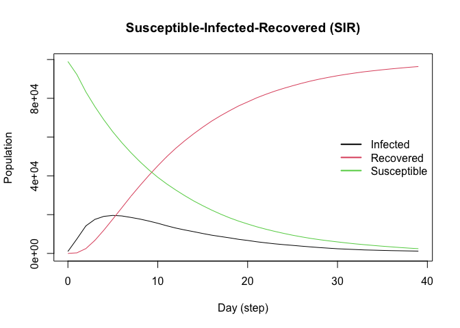
plot_incidence(sir)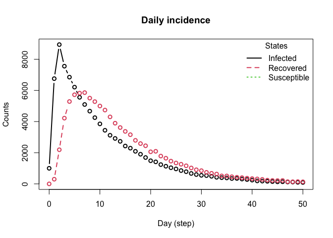
The SEIR model is similar to the SIR model but includes an exposed state. Here, we simulate a population of 10,000 agents with a 0.01 prevalence, a 0.6 transmission rate, a 0.5 recovery rate, and 7 days-incubation period. The population is fully connected, meaning agents can transmit the disease to any other agent:
model_seirconn <- ModelSEIRCONN(
  name                = "COVID-19",
  prevalence          = 0.01,
  n                   = 10000,
  contact_rate        = 10,
  incubation_days     = 7,
  transmission_rate   = 0.1,
  recovery_rate       = 1 / 7
) |> add_virus(
  virus(
    name = "COVID-19 (delta)",
    prevalence = 0.01,
    as_proportion = TRUE,
    prob_infecting = 0.2,
    recovery_rate = 0.6,
    prob_death = 0.5,
    incubation = 7
))

set.seed(132)
run(model_seirconn, ndays = 100)
#> _________________________________________________________________________
#> Running the model...
#> ||||||||||||||||||||||||||||||||||||||||||||||||||||||||||||||||||||||||| done.
summary(model_seirconn)
#> ________________________________________________________________________________
#> ________________________________________________________________________________
#> SIMULATION STUDY
#>
#> Name of the model   : Susceptible-Exposed-Infected-Removed (SEIR) (connected)
#> Population size     : 10000
#> Agents' data        : (none)
#> Number of entities  : 0
#> Days (duration)     : 100 (of 100)
#> Number of viruses   : 2
#> Last run elapsed t  : 77.00ms
#> Last run speed      : 12.90 million agents x day / second
#> Rewiring            : off
#>
#> Global events:
#>  - Update infected individuals (runs daily)
#>
#> Virus(es):
#>  - COVID-19
#>  - COVID-19 (delta)
#>
#> Tool(s):
#>  (none)
#>
#> Model parameters:
#>  - Avg. Incubation days : 7.0000
#>  - Contact rate         : 10.0000
#>  - Prob. Recovery       : 0.1429
#>  - Prob. Transmission   : 0.1000
#>
#> Distribution of the population at time 100:
#>   - (0) Susceptible :  9800 -> 59
#>   - (1) Exposed     :   200 -> 0
#>   - (2) Infected    :     0 -> 0
#>   - (3) Recovered   :     0 -> 9941
#>
#> Transition Probabilities:
#>  - Susceptible  0.95  0.05     -     -
#>  - Exposed         -  0.86  0.14     -
#>  - Infected        -     -  0.79  0.21
#>  - Recovered       -     -     -  1.00
Computing some key statistics
plot(model_seirconn)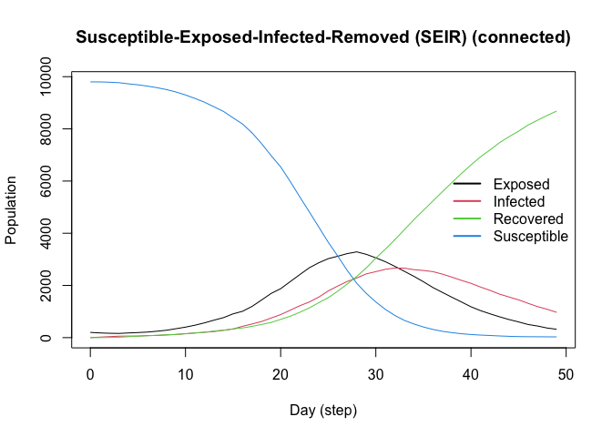
repnum <- get_reproductive_number(model_seirconn)

head(plot(repnum))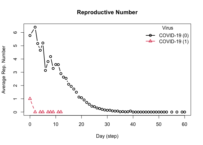
#>   virus_id    virus date      avg   n       sd lb    ub
#> 1        0 COVID-19    0 4.880000 100 4.159157  0 14.05
#> 2        0 COVID-19    2 5.333333   9 4.415880  1 12.60
#> 3        0 COVID-19    3 5.416667  12 3.369875  1 10.45
#> 4        0 COVID-19    4 3.480000  25 2.740438  0  9.80
#> 5        0 COVID-19    5 2.580645  31 2.790152  0  9.00
#> 6        0 COVID-19    6 3.339623  53 3.031523  0 10.40

head(plot_generation_time(model_seirconn))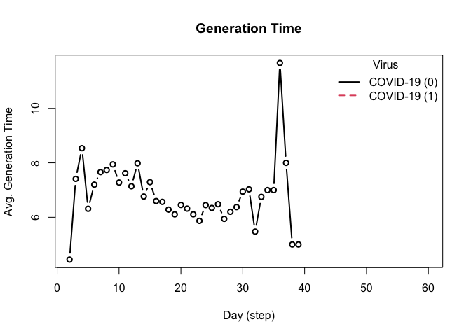
#>   date      avg  n       sd ci_lower ci_upper    virus virus_id
#> 1    0 8.318681 91 5.599363     2.00   20.500 COVID-19        0
#> 2    2 6.888889  9 4.648775     2.20   14.000 COVID-19        0
#> 3    3 5.083333 12 2.503028     3.00    9.725 COVID-19        0
#> 4    4 6.095238 21 3.096849     2.00   12.500 COVID-19        0
#> 5    5 8.173913 23 6.846712     2.55   24.000 COVID-19        0
#> 6 6 7.272727 44 5.332496 2.00 19.000 COVID-19 0This model provides a more complex transmission and recovery pattern
based on agents’ features. With it, we can reflect co-morbidities that
could change the probability of infection and recovery. Here, we
simulate a population including a dataset with two features: an
intercept and a binary variable Female. The probability of
infection and recovery are functions of the intercept and the
Female variables. The following code simulates a population
of 100,000 agents in a small-world network. Each agent is connected to
eight other agents. One percent of the population has the virus, with an
80% chance of transmission. Infected individuals recover at a 0.3
rate:
# Simulating a population of 100,000 agents
set.seed(2223)
n <- 100000

# Agents' features
X <- cbind(
  Intercept = 1,
  Female    = sample.int(2, n, replace = TRUE) - 1
)

coef_infect  <- c(.1, -2, 2)
coef_recover <- rnorm(2)

# Creating the model
model_logit <- ModelSIRLogit(
  "covid2",
  data = X,
  coefs_infect      = coef_infect,
  coefs_recover     = coef_recover,
  coef_infect_cols  = 1L:ncol(X),
  coef_recover_cols = 1L:ncol(X),
  prob_infection = .8,
  recovery_rate = .3,
  prevalence = .01
)

# Adding a small-world population
agents_smallworld(model_logit, n, 8, FALSE, .01)

# Running the model
run(model_logit, 50)
#> _________________________________________________________________________
#> |Running the model...
#> |||||||||||||||||||||||||||||||||||||||||||||||||||||||||||||||||||||||| done.
#> |
plot(model_logit)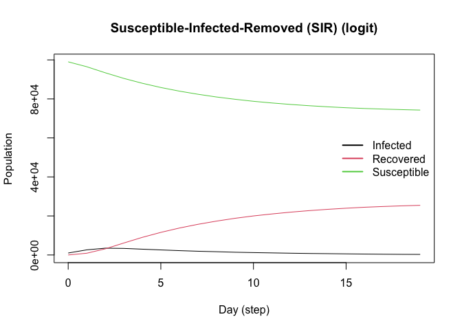
# Females are supposed to be more likely to become infected
rn <- get_reproductive_number(model_logit)

(table(
  X[, "Female"],
  (1:n %in% rn$source)
) |> prop.table())[, 2]
#>       0       1
#> 0.20717 0.22397

# Looking into the agents
get_agents(model_logit)
#> Agents from the model "Susceptible-Infected-Removed (SIR) (logit)":
#> Agent: 0, state: Susceptible (0), Has virus: no, NTools: 0i NNeigh: 8
#> Agent: 1, state: Susceptible (0), Has virus: no, NTools: 0i NNeigh: 8
#> Agent: 2, state: Susceptible (0), Has virus: no, NTools: 0i NNeigh: 8
#> Agent: 3, state: Susceptible (0), Has virus: no, NTools: 0i NNeigh: 8
#> Agent: 4, state: Susceptible (0), Has virus: no, NTools: 0i NNeigh: 8
#> Agent: 5, state: Susceptible (0), Has virus: no, NTools: 0i NNeigh: 8
#> Agent: 6, state: Susceptible (0), Has virus: no, NTools: 0i NNeigh: 8
#> Agent: 7, state: Susceptible (0), Has virus: no, NTools: 0i NNeigh: 8
#> Agent: 8, state: Susceptible (0), Has virus: no, NTools: 0i NNeigh: 8
#> Agent: 9, state: Susceptible (0), Has virus: no, NTools: 0i NNeigh: 8
#> ... 99990 more agents ...This example shows how we can draw a transmission network from a simulation. The following code simulates a population of 500 agents in a small-world network. Each agent is connected to ten other agents. One percent of the population has the virus, with a 50% chance of transmission. Infected individuals recover at a 0.5 rate:
# Creating a SIR model
sir <- ModelSIR(
  name           = "COVID-19",
  prevalence     = .01,
  transmission_rate = .5,
  recovery       = .5
) |>
  # Adding a Small world population
  agents_smallworld(n = 500, k = 10, d = FALSE, p = .01) |>
  # Running the model for 50 days
  run(ndays = 50, seed = 1912)
#> _________________________________________________________________________
#> |Running the model...
#> |||||||||||||||||||||||||||||||||||||||||||||||||||||||||||||||||||||||| done.
#> |

# Transmission network
net <- get_transmissions(sir)
net <- subset(net, source >= 0)

# Plotting
library(epiworldR)
library(netplot)
#> Loading required package: grid
x <- igraph::graph_from_edgelist(
  as.matrix(net[, 2:3]) + 1
)

nplot(x, edge.curvature = 0, edge.color = "gray", skip.vertex = TRUE)
epiworldR supports running multiple simulations using
the run_multiple function. The following code simulates 50
SIR models with 1000 agents each. Each agent is connected to ten other
agents. One percent of the population has the virus, with a 90% chance
of transmission. Infected individuals recover at a 0.1 rate. The results
are saved in a data.frame:
model_sir <- ModelSIRCONN(
  name = "COVID-19",
  prevalence = 0.01,
  n = 1000,
  contact_rate = 2,
  transmission_rate = 0.9, recovery_rate = 0.1
)

# Generating a saver
saver <- make_saver("total_hist", "reproductive")

# Running and printing
# Notice the use of nthread = 2 to run the simulations in parallel
run_multiple(model_sir, ndays = 100, nsims = 50, saver = saver, nthread = 2)
#> Starting multiple runs (50) using 2 thread(s)
#> _________________________________________________________________________
#> _________________________________________________________________________
#> ||||||||||||||||||||||||||||||||||||||||||||||||||||||||||||||||||||||||| done.

# Retrieving the results
ans <- run_multiple_get_results(model_sir)

head(ans$total_hist)
#>   sim_num date nviruses       state counts
#> 1       1    0        1 Susceptible    990
#> 2       1    0        1    Infected     10
#> 3       1    0        1   Recovered      0
#> 4       1    1        1 Susceptible    973
#> 5       1    1        1    Infected     27
#> 6       1    1        1   Recovered      0
head(ans$reproductive)
#>   sim_num virus_id    virus source source_exposure_date rt
#> 1       1        0 COVID-19    683                    9  0
#> 2       1        0 COVID-19    983                    8  0
#> 3       1        0 COVID-19    875                    8  0
#> 4       1        0 COVID-19    801                    8  0
#> 5       1        0 COVID-19    770                    8  0
#> 6       1        0 COVID-19    758                    8  0

plot(ans$reproductive)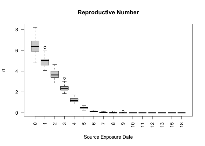
The virtual INSNA Sunbelt 2023 session can be found here: https://github.com/UofUEpiBio/epiworldR-workshop/tree/sunbelt2023-virtual
The in-person INSNA Sunbelt 2023 session can be found here: https://github.com/UofUEpiBio/epiworldR-workshop/tree/sunbetl2023-inperson
If you use epiworldR in your research, please cite it as
follows:
citation("epiworldR")
#> To cite epiworldR in publications use:
#>
#>   Meyer, Derek and Vega Yon, George (2023). epiworldR: Fast Agent-Based
#>   Epi Models. Journal of Open Source Software, 8(90), 5781,
#>   https://doi.org/10.21105/joss.05781
#>
#> And the actual R package:
#>
#>   Meyer D, Pulsipher A, Vega Yon G (2025). _epiworldR: Fast Agent-Based
#>   Epi Models_. R package version 0.11.3.0,
#>   <https://github.com/UofUEpiBio/epiworldR>.
#>
#> To see these entries in BibTeX format, use 'print(<citation>,
#> bibtex=TRUE)', 'toBibtex(.)', or set
#> 'options(citation.bibtex.max=999)'.Several alternatives to epiworldR exist and provide
researchers with a range of options, each with its own unique features
and strengths, enabling the exploration and analysis of infectious
disease dynamics through agent-based modeling. Below is a manually
curated table of existing alternatives, including ABM [@ABM], abmR [@abmR], cystiSim [@cystiSim], villager
[@villager], and
RNetLogo [@RNetLogo].
| Package | Multiple Viruses | Multiple Tools | Multiple Runs | Global Actions | Built-In Epi Models | Dependencies | Activity |
|---|---|---|---|---|---|---|---|
| epiworldR | yes | yes | yes | yes | yes |  |
|
| ABM | - | - | - | yes | yes |  |
|
| abmR | - | - | yes | - | - |  |
|
| cystiSim | - | yes | yes | - | - |  |
|
| villager | - | - | - | yes | - |  |
|
| RNetLogo | - | yes | yes | yes | - |  |
You may want to check out other R packages for agent-based modeling:
ABM,
abmR,
cystiSim,
villager, and
RNetLogo.
We welcome contributions to the epiworldR package! If you would like to contribute, please review our development guidelines before creating a pull request.
The epiworldR project is released with a Contributor Code of Conduct. By contributing to this project, you agree to abide by its terms.
These binaries (installable software) and packages are in development.
They may not be fully stable and should be used with caution. We make no claims about them.