The hardware and bandwidth for this mirror is donated by METANET, the Webhosting and Full Service-Cloud Provider.
If you wish to report a bug, or if you are interested in having us mirror your free-software or open-source project, please feel free to contact us at mirror[@]metanet.ch.
![]()
The goal of fEGarch is to provide easy access to a broad
family of exponential generalized autoregressive conditional
heteroskedasticity (EGARCH) models both with either short or long
memory. The six most common conditional distributions, i.e. a normal
distribution, a t-distribution, a generalized error distribution, and
the skewed variants of those three, are available. Furthermore, we
introduce the average Laplace distribution and its skewed variant as
newly selectable conditional distributions. Overall, the EGARCH family
models are a strong competition to well-established GARCH-type models
and provide new ways to estimate conditional volatilities, while making
the prominent EGARCH and fractionally integrated EGARCH (FIEGARCH)
available as special cases. For convenience and the purpose of
comparison, fractionally integrated asymmetric power ARCH (FIAPARCH),
fractionally integrated Glosten-Jagannathan-Runkle GARCH (FIGJR-GARCH),
fractionally integrated threshold GARCH (FITGARCH) and fractionally
integrated GARCH (FIGARCH) models are available as well as their
short-memory variants (APARCH, GJR-GARCH, TGARCH, GARCH). Throughout,
the estimation method is quasi-maximum-likelihood estimation
(conditioned on presample values).
You can install the current version of the package from CRAN with:
install.packages("fEGarch")This is a basic example which shows you how to fit a model of the EGARCH family to the Standard and Poor’s 500 daily log-returns.
At first, specify a model from the EGARCH family using
fEGarch_spec().
library(fEGarch)

### 1. Set model specification via "fEGarch_spec()"
spec1 <- fEGarch_spec(
  model_type = "egarch",       # the basic model type among EGARCH and
                               # Log-GARCH as subclasses of the broad
                               # EGARCH family;
  orders = c(1, 1),            # the model orders;
  long_memo = TRUE,            # include long memory?;
  cond_dist = "norm",          # the conditional distribution;
  powers = c(0, 0),            # powers of the asymmetry and magnitude terms, respectively;
  modulus = c(TRUE, TRUE)      # whether or not to apply a modulus transformation
                               # to the asymmetry and magnitude terms, respectively
)

# -> Specification now aligns with that of FIMLog-GARCH(1, 1) with
#    conditional normal distribution
Afterwards, use the model specification returned by
fEGarch_spec() together with your data object and apply the
estimation function fEGarch() to them. As can be seen, the
package also imports and exports the pipe operator %>%
of the magrittr package for a simplified coding workflow.
Note that the object SP500 in the package is already
formatted as an object of class "zoo", which also already
contains information about the observation time points. This will later
on automate the x-axis formatting in automated plots created with the
package.
### 2. Use specification to fit model to data
rt <- SP500
model1 <- spec1 %>%
  fEGarch(rt)
model1
#> *************************************
#> *     Fitted EGARCH Family Model    *
#> *************************************
#>
#> Type: egarch
#> Orders: (1, 1)
#> Modulus: (TRUE, TRUE)
#> Powers: (0, 0)
#> Long memory: TRUE
#> Cond. distribution: norm
#>
#> ARMA orders (cond. mean): (0, 0)
#> Long memory (cond. mean): FALSE
#>
#> Scale estimation: FALSE
#>
#> Fitted parameters:
#>
#>               par     se     tval   pval
#> mu         0.0003 0.0000  23.9025 0.0000
#> omega_sig -8.6599 0.1271 -68.1095 0.0000
#> phi1       0.8680 0.0227  38.1874 0.0000
#> kappa     -0.2362 0.0146 -16.1675 0.0000
#> gamma      0.3194 0.0209  15.2989 0.0000
#> d          0.2754 0.0377   7.3053 0.0000
#>
#> Information criteria (parametric part):
#> AIC: -6.4945, BIC: -6.4880
A convenient way to implement various specific model specifications
is available via a selection of wrappers for
fEGarch_spec(). They all only have the function arguments
orders and cond_dist from
fEGarch_spec().
### 3. Use shortcuts for submodel specifications
spec2 <- megarch_spec()         # Specification for MEGARCH
spec3 <- mloggarch_spec()       # Specification for MLog-GARCH
spec4 <- egarch_spec()          # Specification for EGARCH
spec5 <- loggarch_spec()        # Specification for Log-GARCH
spec6 <- fiegarch_spec()        # Specification for FIEGARCH
spec7 <- filoggarch_spec()      # Specification for FILog-GARCH
spec8 <- fimloggarch_spec()     # Specification for FIMLog-GARCH
spec9 <- fimegarch_spec()       # Specification for FIMEGARCH

# -> All with adjustable arguments "orders" and "cond_dist".

spec10 <- megarch_spec(orders = c(2, 1), cond_dist = "std")
They can all be used in fEGarch(). In the following, the
previously created model specification spec10 is considered
for the log-returns. The other specifications can be applied
analogously.
model10 <- spec10 %>%
  fEGarch(rt)   # ... and so on for other specifications
model10
#> *************************************
#> *     Fitted EGARCH Family Model    *
#> *************************************
#>
#> Type: egarch
#> Orders: (2, 1)
#> Modulus: (TRUE, FALSE)
#> Powers: (0, 1)
#> Long memory: FALSE
#> Cond. distribution: std
#>
#> ARMA orders (cond. mean): (0, 0)
#> Long memory (cond. mean): FALSE
#>
#> Scale estimation: FALSE
#>
#> Fitted parameters:
#>
#>               par     se     tval   pval
#> mu         0.0004 0.0001   4.6743 0.0000
#> omega_sig -9.4104 0.1170 -80.4515 0.0000
#> phi1       0.9762 0.0719  13.5832 0.0000
#> phi2      -0.0000 0.0707  -0.0000 1.0000
#> kappa     -0.2946 0.0266 -11.0709 0.0000
#> gamma      0.1651 0.0150  10.9784 0.0000
#> df         7.0906 0.6071  11.6790 0.0000
#>
#> Information criteria (parametric part):
#> AIC: -6.5391, BIC: -6.5316
As a further extension, dual-models with autoregressive
moving-average (ARMA) model or fractionally integrated ARMA (FARIMA /
ARFIMA) model in the conditional mean simultaneously with error process
from the EGARCH family can be defined and estimated. For this purpose,
the mean_spec() function must be utilized in addition to
the previous steps.
spec_egarch <- egarch_spec()
spec_arma <- mean_spec(
  orders = c(1, 1),     # ARMA orders
  long_memo = FALSE,    # Long-memory?
  include_mean = TRUE   # Estimate uncond. mean?
)
model11 <- spec_egarch %>%
  fEGarch(rt, meanspec = spec_arma)
model11
#> *************************************
#> *     Fitted EGARCH Family Model    *
#> *************************************
#>
#> Type: egarch
#> Orders: (1, 1)
#> Modulus: (FALSE, FALSE)
#> Powers: (1, 1)
#> Long memory: FALSE
#> Cond. distribution: norm
#>
#> ARMA orders (cond. mean): (1, 1)
#> Long memory (cond. mean): FALSE
#>
#> Scale estimation: FALSE
#>
#> Fitted parameters:
#>
#>               par     se      tval   pval
#> mu         0.0003 0.0000    7.9547 0.0000
#> ar1        0.2448 0.0082   29.8485 0.0000
#> ma1       -0.2944 0.0081  -36.3976 0.0000
#> omega_sig -9.1718 0.0643 -142.5974 0.0000
#> phi1       0.9719 0.0027  359.9865 0.0000
#> kappa     -0.1333 0.0078  -17.1204 0.0000
#> gamma      0.1608 0.0124   12.9570 0.0000
#>
#> Information criteria (parametric part):
#> AIC: -6.4975, BIC: -6.4899
Yet another alternative is the fitting of semiparametric extensions of conditional variance models. Modelling the conditional mean simultaneously via an ARMA or FARIMA model in such a semiparametric extension is currently not possible. The nonparametric, smooth scale function reflecting the unconditional standard deviation over time is estimated using automated local polynomial regression with two different algorithms for short-memory and long-memory errors.
model12 <- fiegarch_spec(cond_dist = "std") %>%
  fEGarch(rt, use_nonpar = TRUE)
model12
#> *************************************
#> *     Fitted EGARCH Family Model    *
#> *************************************
#>
#> Type: egarch
#> Orders: (1, 1)
#> Modulus: (FALSE, FALSE)
#> Powers: (1, 1)
#> Long memory: TRUE
#> Cond. distribution: std
#>
#> ARMA orders (cond. mean): (0, 0)
#> Long memory (cond. mean): FALSE
#>
#> Scale estimation: TRUE (poly_order = 3; bandwidth = 0.1493)
#>
#> Fitted parameters:
#>
#>               par     se     tval   pval
#> omega_sig -0.5382 0.1812  -2.9698 0.0030
#> phi1       0.7907 0.0701  11.2815 0.0000
#> kappa     -0.1519 0.0126 -12.0240 0.0000
#> gamma      0.1236 0.0121  10.2397 0.0000
#> d          0.3963 0.0846   4.6867 0.0000
#> df         7.5375 0.6688  11.2706 0.0000
#>
#> Information criteria (parametric part):
#> AIC: 2.4655, BIC: 2.4719
plot(cbind("Standardized" = (rt - mean(rt)) / sd(rt),
           "Scale-adjusted" = (rt - mean(rt)) / model12@scale_fun),
     xlab = "Year",
     main = "Standardized log-returns and their scale-adjusted version")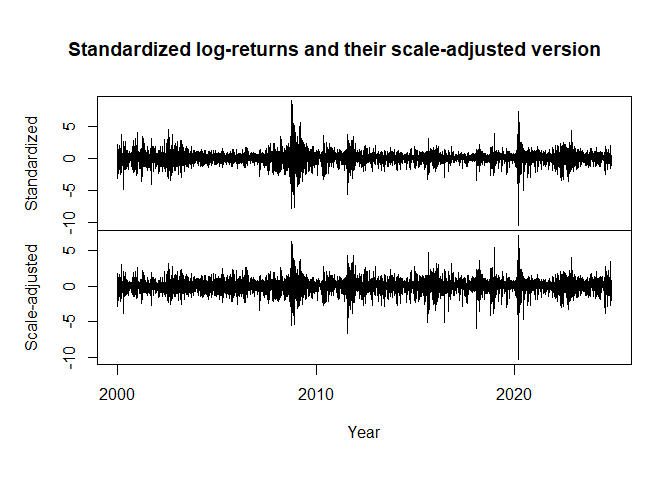
The estimated volatility is then the product of the estimated scale function and the estimated conditional standard deviation both obtained at the corresponding time point.
Note that the returned AIC and BIC values are only valid for parametric model parts and are, in case of a semiparametric model, based on the scale-adjusted returns. A direct comparison of AIC and BIC values between purely parametric and semiparametric models is therefore not possible.
Estimation objects returned by fEGarch() contain several
elements. They can be either accessed through the operator
@ or via specific accessor functions named after the
corresponding elements in the output object. To access the fitted
conditional standard deviations, the fitted conditional means and the
standardized residuals, the package also alternatively provides methods
sigma(), fitted() and
residuals(), respectively.
sigt1 <- sigt(model1)
sigt10 <- model10@sigt
TS <- cbind(
  "Log-returns" = rt,
  "Model 1" = sigt1,
  "Model 10" = sigt10
)
If the input data is formatted as a time series object of class
"zoo", fEGarch() applies the same formatting
to all output series in its returned object, also to the estimated
conditional standard deviations.
plot(TS, xlab = "Year", main = "Example application")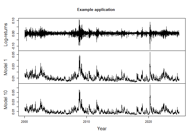
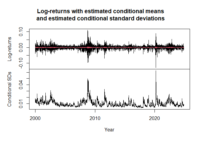
Furthermore, also the conditional means of the previously estimated
model11 object can be obtained.
cond11 <- cmeans(model11)
sig11 <- sigt(model11)

plot.zoo <- get("plot.zoo", envir = asNamespace("zoo"))

obj <- cbind(
  "Log-returns" = rt,
  "Conditional means" = cond11,
  "Conditional SDs" = sig11
)
plot.zoo(obj, screens = c(1, 1, 2), col = c(1, 2, 1),
  main = paste0(
    "Log-returns with estimated conditional means\n",
    "and estimated conditional standard deviations"
  ),
  xlab = "Year"
)
The fEGarch package also allows for the estimation of
FIAPARCH and FIGARCH models, however, currently only with fixed model
orders p = q = 1. For these two models, there are two fitting functions
figarch() and fiaparch() available without any
preceding model specification steps. Model specifications can be made
via arguments within these functions directly. Alternatively, the
wrapper garchm_estim() can be used to select and fit a
GARCH-type model (not belonging to the EGARCH family).
model_fiaparch <- rt %>%
  fiaparch(orders = c(1, 1), cond_dist = "std")
model_fiaparch2 <- rt %>%
  garchm_estim(model = "fiaparch", orders = c(1, 1), cond_dist = "std")
model_figarch <- rt %>%
  figarch(orders = c(1, 1), cond_dist = "std")
model_figarch
#> *************************************
#> *        Fitted FIGARCH Model       *
#> *************************************
#>
#> Type: figarch
#> Orders: (1, 1)
#> Long memory: TRUE
#> Cond. distribution: std
#>
#> ARMA orders (cond. mean): (0, 0)
#> Long memory (cond. mean): FALSE
#>
#> Scale estimation: FALSE
#>
#> Fitted parameters:
#>
#>          par     se    tval   pval
#> mu    0.0008 0.0001  8.3454 0.0000
#> omega 0.0000 0.0000  3.3310 0.0009
#> phi1  0.0261 0.0328  0.7944 0.4269
#> beta1 0.6088 0.0557 10.9287 0.0000
#> d     0.6437 0.0571 11.2682 0.0000
#> df    6.4693 0.4858 13.3159 0.0000
#>
#> Information criteria (parametric part):
#> AIC: -6.5033, BIC: -6.4968
sigt_fiaparch <- sigt(model_fiaparch)
sigt_figarch <- sigt(model_figarch)
TS2 <- cbind(
"Log-returns" = rt,
"FIMLog-GARCH" = sigt1,
"MEGARCH" = sigt10,
"FIAPARCH" = sigt_fiaparch,
"FIGARCH" = sigt_figarch
)
plot(TS2, xlab = "Year", main = "Another example application", nc = 1)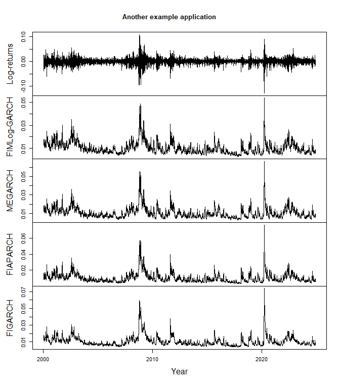
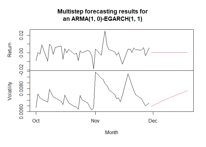
The package provides the two commands predict() and
predict_roll() to compute, given a fitted model from the
package, either multistep out-of-sample point forecasts of the
conditional standard deviation (and of the conditional mean) or rolling
point forecasts (of arbitrarily selectable step size) of the conditional
standard deviation (and of the conditional mean) over some reserved test
sample. Setting refit_after to a positive integer in
predict_roll() forces refitting of the model after that
number of observations before continuing with the rolling forecasts.
For multistep forecasts into the future, consider
predict and its argument n.ahead.
new_model <- egarch_spec() %>%
  fEGarch(rt, meanspec = mean_spec(orders = c(1, 0)))
new_model
#> *************************************
#> *     Fitted EGARCH Family Model    *
#> *************************************
#>
#> Type: egarch
#> Orders: (1, 1)
#> Modulus: (FALSE, FALSE)
#> Powers: (1, 1)
#> Long memory: FALSE
#> Cond. distribution: norm
#>
#> ARMA orders (cond. mean): (1, 0)
#> Long memory (cond. mean): FALSE
#>
#> Scale estimation: FALSE
#>
#> Fitted parameters:
#>
#>               par     se      tval   pval
#> mu         0.0003 0.0000   11.5305 0.0000
#> ar1       -0.0498 0.0026  -19.0265 0.0000
#> omega_sig -9.1673 0.0623 -147.2011 0.0000
#> phi1       0.9719 0.0027  362.0598 0.0000
#> kappa     -0.1353 0.0077  -17.4776 0.0000
#> gamma      0.1600 0.0124   12.9308 0.0000
#>
#> Information criteria (parametric part):
#> AIC: -6.4976, BIC: -6.4911
fc <- new_model %>%
  predict(n.ahead = 20)
plot(
  cbind(
    "Return" = cmeans(fc),
    "Volatility" = sigt(fc),
    "Return_in" = window(new_model@rt, start = as.Date("2024-10-01")),
    "Vol_in" = window(sigt(new_model), start = as.Date("2024-10-01"))
  ),
  screens = c(1, 2, 1, 2),
  col = c(2, 2, 1, 1),
  main = "Multistep forecasting results for\nan ARMA(1, 0)-EGARCH(1, 1)",
  xlab = "Month"
)
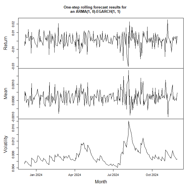
Rolling point forecasts can be computed using
predict_roll, if previously in the model estimation step
observations were reserved for testing using the argument
n_test.
new_model <- egarch_spec() %>%
  fEGarch(rt, meanspec = mean_spec(orders = c(1, 0)), n_test = 250)
new_model
#> *************************************
#> *     Fitted EGARCH Family Model    *
#> *************************************
#>
#> Type: egarch
#> Orders: (1, 1)
#> Modulus: (FALSE, FALSE)
#> Powers: (1, 1)
#> Long memory: FALSE
#> Cond. distribution: norm
#>
#> ARMA orders (cond. mean): (1, 0)
#> Long memory (cond. mean): FALSE
#>
#> Scale estimation: FALSE
#>
#> Fitted parameters:
#>
#>               par     se      tval   pval
#> mu         0.0003 0.0001    2.7576 0.0058
#> ar1       -0.0517 0.0135   -3.8211 0.0001
#> omega_sig -9.1586 0.0800 -114.4542 0.0000
#> phi1       0.9727 0.0027  354.9871 0.0000
#> kappa     -0.1359 0.0080  -16.9483 0.0000
#> gamma      0.1591 0.0126   12.5910 0.0000
#>
#> Information criteria (parametric part):
#> AIC: -6.4792, BIC: -6.4725
fc2 <- new_model %>%
  predict_roll(refit_after = 25)
plot(
  cbind(
    "Return" = new_model@test_obs,
    "Mean" = cmeans(fc2),
    "Volatility" = sigt(fc2)
  ),
  screens = c(1, 2, 3),
  main = "One-step rolling forecast results for\nan ARMA(1, 0)-EGARCH(1, 1)",
  xlab = "Month"
)
The results from one-step rolling point forecasts for the conditional
mean and the conditional standard deviation for test time points can be
used for common backtesting approaches. first and foremost, the
resulting object from a call to predict_roll can be fed to
measure_risk to compute value at risk (VaR) and expected
shortfall (ES) following those forecasts and the underlying conditional
distribution.
risk <- fc2 %>%
  measure_risk()
By default, the 97.5% and the 99% VaR and ES will be computed. A
plotting method (also additionally available as autoplot
for compatibility with the ggplot2 framework) allows for
plotting the test returns together with the VaR and ES of a selected
confidence level from the output of measure_risk.
risk %>%
  plot(which = 0.975, xlab = "Month")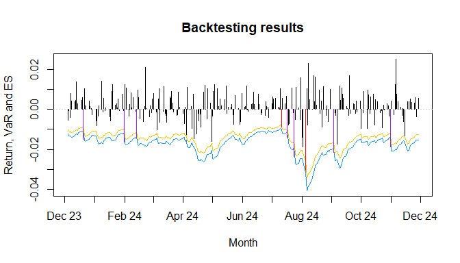
As can be seen, the breaches of the VaR are automatically highlighted
through the colors red and purple. Breaches of the ES (and therefore
implied also of the VaR) are shown through the color purple alone.
Furthermore, time series formatting of "zoo" objects is
kept for simplified formatting of the x-axis.
Moreover, a test suite consisting of traffic light tests for VaR and
ES and of coverage and independence tests can be applied using
backtest_suite on the output of measure_risk.
Note that test results (rejecting or not rejecting the null hypothesis)
for the coverage and independence tests are stated under consideration
of a 5-percent significance level; however, other significance levels
can be considered as well via the also given p-values for each of these
tests.
risk %>%
  backtest_suite()
#>
#> ***********************
#> * Traffic light tests *
#> ***********************
#>
#> VaR results:
#> ************
#>
#> Conf. level: 0.975
#> Breaches: 9
#> Cumul. prob.: 0.9005
#> Zone: Green zone
#>
#> Conf. level: 0.99
#> Breaches: 7
#> Cumul. prob.: 0.9960
#> Zone: Yellow zone
#>
#>
#> ES results:
#> ***********
#>
#> Conf. level: 0.975
#> Severity of breaches: 6.9862
#> Cumul. prob.: 0.9965
#> Zone: Yellow zone
#>
#> Conf. level: 0.99
#> Severity of breaches: 4.9905
#> Cumul. prob.: 1.0000
#> Zone: Red zone
#>
#>
#>
#> *******************************
#> * Weighted Absolute Deviation *
#> *******************************
#>
#> Following 99%-VaR, 97.5%-VaR and 97.5%-ES.
#>
#> WAD: 3.4756
#>
#>
#> ***************************************
#> * Unconditional coverage test for VaR *
#> ***************************************
#>
#> H0: true share of covered observations = theoretical share of VaR
#>
#> Conf. level: 0.975
#> Breaches: 9
#> Test statistic: 1.0947
#> p-value: 0.2954
#> Decision: Do not reject H0
#>
#> Conf. level: 0.99
#> Breaches: 7
#> Test statistic: 5.4970
#> p-value: 0.0190
#> Decision: Reject H0
#>
#>
#> *****************************
#> * Independence test for VaR *
#> *****************************
#>
#> H0: true share of covered observations independent
#>     of breach or no breach at previous time point
#>
#> Conf. level: 0.975
#> Breaches: 9
#> Test statistic: 0.6752
#> p-value: 0.4113
#> Decision: Do not reject H0
#>
#> Conf. level: 0.99
#> Breaches: 7
#> Test statistic: 0.4050
#> p-value: 0.5245
#> Decision: Do not reject H0
#>
#>
#> *************************************
#> * Conditional coverage test for VaR *
#> *************************************
#>
#> H0: true share of covered observations simultaneously
#>     independent of breach or no breach at previous time point
#>     and equal to theoretical share of VaR
#>
#> Conf. level: 0.975
#> Breaches: 9
#> Test statistic: 1.7927
#> p-value: 0.4081
#> Decision: Do not reject H0
#>
#> Conf. level: 0.99
#> Breaches: 7
#> Test statistic: 5.9388
#> p-value: 0.0513
#> Decision: Do not reject H0
Ultimately, the package is also capable of computing loss functions based on VaR and ES. For detailed description of those loss functions, see the manual of the package.
# Output suppressed to save space
risk %>%
  loss_functions(penalty = 1e-04)
A slightly better model regarding VaR and ES forecasting for this particular example could be implemented and checked as follows.
# Fit and check an Semi-Log-GARCH(1, d, 1) with
# conditional skew-t-distribution
new_model2 <- loggarch_spec(cond_dist = "sstd") %>%
  fEGarch(rt, n_test = 250, use_nonpar = TRUE)

risk_nm2 <- new_model2 %>%
  predict_roll(refit_after = 25) %>%
  measure_risk()

risk_nm2 %>%
  backtest_suite()
#>
#> ***********************
#> * Traffic light tests *
#> ***********************
#>
#> VaR results:
#> ************
#>
#> Conf. level: 0.975
#> Breaches: 9
#> Cumul. prob.: 0.9005
#> Zone: Green zone
#>
#> Conf. level: 0.99
#> Breaches: 3
#> Cumul. prob.: 0.7581
#> Zone: Green zone
#>
#>
#> ES results:
#> ***********
#>
#> Conf. level: 0.975
#> Severity of breaches: 4.2807
#> Cumul. prob.: 0.7905
#> Zone: Green zone
#>
#> Conf. level: 0.99
#> Severity of breaches: 1.3067
#> Cumul. prob.: 0.5248
#> Zone: Green zone
#>
#>
#>
#> *******************************
#> * Weighted Absolute Deviation *
#> *******************************
#>
#> Following 99%-VaR, 97.5%-VaR and 97.5%-ES.
#>
#> WAD: 1.0098
#>
#>
#> ***************************************
#> * Unconditional coverage test for VaR *
#> ***************************************
#>
#> H0: true share of covered observations = theoretical share of VaR
#>
#> Conf. level: 0.975
#> Breaches: 9
#> Test statistic: 1.0947
#> p-value: 0.2954
#> Decision: Do not reject H0
#>
#> Conf. level: 0.99
#> Breaches: 3
#> Test statistic: 0.0949
#> p-value: 0.7580
#> Decision: Do not reject H0
#>
#>
#> *****************************
#> * Independence test for VaR *
#> *****************************
#>
#> H0: true share of covered observations independent
#>     of breach or no breach at previous time point
#>
#> Conf. level: 0.975
#> Breaches: 9
#> Test statistic: 0.6752
#> p-value: 0.4113
#> Decision: Do not reject H0
#>
#> Conf. level: 0.99
#> Breaches: 3
#> Test statistic: 0.0732
#> p-value: 0.7868
#> Decision: Do not reject H0
#>
#>
#> *************************************
#> * Conditional coverage test for VaR *
#> *************************************
#>
#> H0: true share of covered observations simultaneously
#>     independent of breach or no breach at previous time point
#>     and equal to theoretical share of VaR
#>
#> Conf. level: 0.975
#> Breaches: 9
#> Test statistic: 1.7927
#> p-value: 0.4081
#> Decision: Do not reject H0
#>
#> Conf. level: 0.99
#> Breaches: 3
#> Test statistic: 0.1722
#> p-value: 0.9175
#> Decision: Do not reject H0resids <- new_model@etat
test_obs <- new_model@test_obs
sigt <- fc2@sigt
cmeans <- fc2@cmeansAssume now that the objects resids,
test_obs, sigt and cmeans reflect
the in-sample standardized residuals obtained from some model, the test
returns, one-step rolling point forecasts of the conditional standard
deviation for the same test period and the one-step rolling point
forecasts of the conditional mean for the same test period,
respectively. Furthermore, also assume that they were not obtained
through a parametric (or semiparametric) GARCH-type model but through
some fully nonparametric idea like for example a neural network. To be
precise, the forecasts would need to be obtained without model
refitting. Given those series, the fEGarch package provides
a simple way to compute and backtest VaR and ES even for such
nonparametric approaches (without model refitting).
opt_dist <- resids %>%
  find_dist(fix_mean = 0, fix_sdev = 1, criterion = "bic")
opt_dist
#> *************************************
#> *         Fitted Distribution       *
#> *************************************
#>
#> Distribution: sald
#> Fixed: 0 (mean), 1 (sdev)
#>
#> Fitted parameters:
#>
#>         par     se    tval   pval
#> P    2.0000     NA      NA     NA
#> skew 0.8580 0.0142 60.4712 0.0000
#>
#> Information criteria:
#> AIC: 2.7877, BIC: 2.7900
risk_obj <- opt_dist %>%
  measure_risk(test_obs = test_obs, sigt = sigt, cmeans = cmeans)
find_dist() uses maximum-likelihood estimation on the
in-sample standardized residual series to find the best distribution
among the eight available innovation distributions in this package
following either the BIC (the default) or the AIC. This returns an
object of class "fEGarch_distr_est", for which there is a
special method of measure_risk(). Therefore, to compute the
VaR and ES forecasts, feed the output of find_dist() to
measure_risk() while also supplying the function with the
objects test_obs, sigt and
cmeans. The output is now formatted identically to that of
the measure_risk() method applied to the output of
predict_roll() for GARCH-type models and can be treated the
same as before.
risk_obj %>%
  plot(which = 0.975, xlab = "Month")
# Inclusion of the output is omitted here to save space.
risk_obj %>%
backtest_suite()
# Inclusion of the output is omitted here to save space.The package allows for the implementation of dual long-memory models
(long-memory in mean together with long-memory in volatility), which can
be useful for applications to non-return data as well. In the following,
a FARIMA(0, d ,1)-FIMLog-GARCH(1, d, 1) model (with conditional skewed
average Laplace distribution) is applied to the data
UKinflation, which contains monthly UK inflation rates over
time and which is provided in the package.
xt <- UKinflation
dual_lm_model <- fimloggarch_spec(cond_dist = "sald") %>%
  fEGarch(xt, meanspec = mean_spec(orders = c(0, 1), long_memo = TRUE))
dual_lm_model
#> *************************************
#> *     Fitted EGARCH Family Model    *
#> *************************************
#>
#> Type: egarch
#> Orders: (1, 1)
#> Modulus: (TRUE, TRUE)
#> Powers: (0, 0)
#> Long memory: TRUE
#> Cond. distribution: sald
#>
#> ARMA orders (cond. mean): (0, 1)
#> Long memory (cond. mean): TRUE
#>
#> Scale estimation: FALSE
#>
#> Fitted parameters:
#>
#>               par     se     tval   pval
#> mu         0.4038 0.0423   9.5449 0.0000
#> ma1       -0.0054 0.0018  -2.9887 0.0028
#> D          0.2322 0.0076  30.6137 0.0000
#> omega_sig -1.4809 0.0934 -15.8469 0.0000
#> phi1       0.7217 0.1246   5.7938 0.0000
#> kappa      0.3394 0.0989   3.4302 0.0006
#> gamma      0.0331 0.1021   0.3242 0.7458
#> d          0.1574 0.1314   1.1981 0.2309
#> P          1.0000     NA       NA     NA
#> skew       1.2916 0.0690  18.7204 0.0000
#>
#> Information criteria (parametric part):
#> AIC: 1.3413, BIC: 1.4208

oldpar <- par(no.readonly = TRUE)
par(mfrow = c(2, 1), cex = 1, mar = c(4, 4, 3, 2) + 0.1)

ts.plot(xt, fitted(dual_lm_model), col = c("grey64", "red"),
        xlab = "Year", ylab = "Inflation rate",
        main = "UK inflation rate together with conditional means")
plot.ts(sigma(dual_lm_model), xlab = "Year",
        ylab = "Conditional standard deviation",
        main = "Conditional volatility of UK inflation")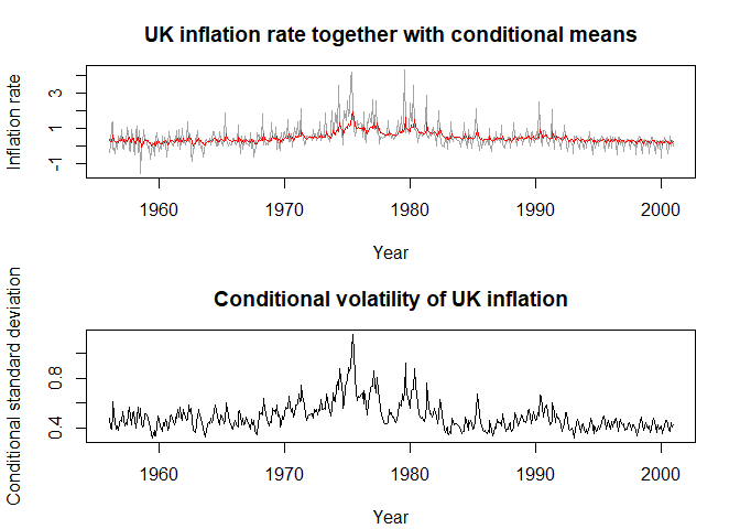
par(oldpar)The main functions of the package are:
fEGarch_spec(): general EGARCH family model
specification,
fEGarch(): fitting function for models of the
broader EGARCH family,
garchm_estim(): GARCH-type model fitting selectable
from standard GARCH, GJR-GARCH, TGARCH, APARCH, FIGARCH, FIGJR-GARCH,
FITGARCH and FIAPARCH.
fEGarch_sim(): EGARCH family simulation,
fiaparch_sim(): FIAPARCH simulation,
figarch_sim(): FIGARCH simulation,
figjrgarch_sim(): FIGJR-GARCH simulation,
fitgarch_sim(): FITGARCH simulation,
aparch_sim(): APARCH simulation,
garch_sim(): GARCH simulation,
gjrgarch_sim(): GJR-GARCH simulation,
tgarch_sim(): TGARCH simulation,
mean_spec(): ARMA or FARIMA model specification for
simultaneously modelling the conditional mean,
predict(): a forecasting method to compute multistep
point forecasts of the conditional mean and the conditional standard
deviation following one of the package’s fitted models,
predict_roll(): a method to compute rolling point
forecasts of the conditional mean and the conditional standard deviation
over a test set following one of the package’s fitted models.
measure_risk(): given certain input objects with
information about (forecasts of) conditional standard deviation and
conditional mean, computes the corresponding (forecasts of) VaR and
ES.
backtest_suite(): a collection of tests for
backtesting of VaR and ES.
find_dist(): fits all eight distributions considered
in this package to a supposed iid series and selects the best fitted
distribution following either BIC (the default) or AIC.
The package, however, provides many other useful functions to discover.
The package contains an example time series SP500,
namely the Standard and Poor’s 500 daily log-return series from January
04, 2000, until November 30, 2024, obtained from Yahoo Finance. The
series is formatted as a time series object of class "zoo".
Furthermore, it contains the dataset UKinflation with the
monthly inflation rate of the UK from January 1956 to December 2000.
This second series is formatted as a time series of class
"ts".
Dominik Schulz (Department Economics, Paderborn University, Germany) (Author, Maintainer)
Yuanhua Feng (Department Economics, Paderborn University, Germany) (Author)
Christian Peitz (Financial Intelligence Unit, German Government) (Author)
Oliver Kojo Ayensu (Department Economics, Paderborn University, Germany) (Author)
For questions, bug reports, etc., please contact the maintainer Mr. Dominik Schulz via dominik.schulz@uni-paderborn.de.
If you are using this software for your publication, please consider citing
These binaries (installable software) and packages are in development.
They may not be fully stable and should be used with caution. We make no claims about them.