The hardware and bandwidth for this mirror is donated by METANET, the Webhosting and Full Service-Cloud Provider.
If you wish to report a bug, or if you are interested in having us mirror your free-software or open-source project, please feel free to contact us at mirror[@]metanet.ch.
The ‘fastglm’ package is a re-write of glm() using
RcppEigen designed to be computationally efficient and
algorithmically stable.
Install the development version using the devtools package:
devtools::install_github("jaredhuling/fastglm")or by cloning and building using R CMD INSTALL
Load the package:
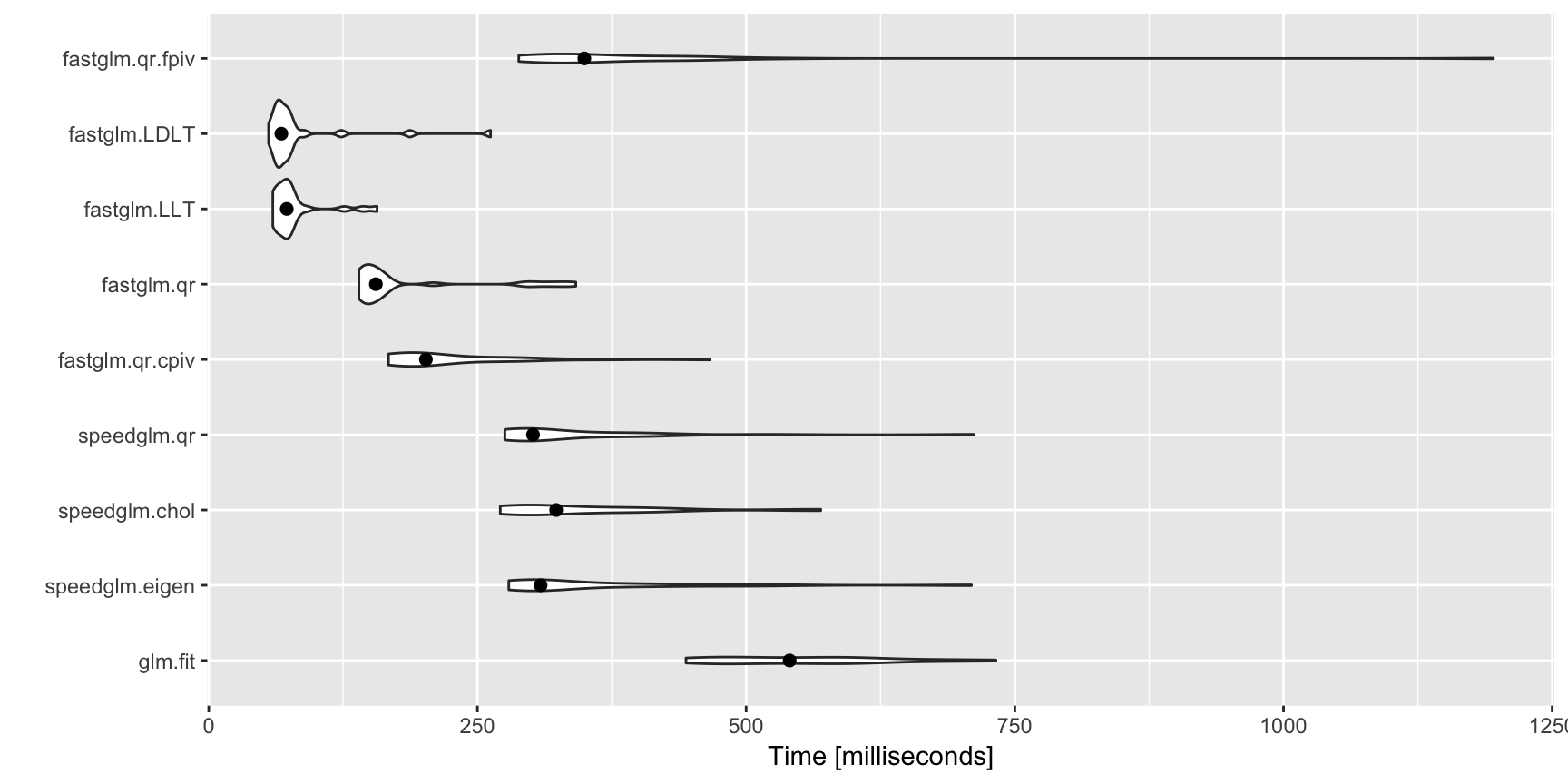
library(fastglm)A (not comprehensive) comparison with glm.fit() and
speedglm.wfit():
library(speedglm)
library(microbenchmark)
library(ggplot2)

set.seed(123)
n.obs  <- 10000
n.vars <- 100
x <- matrix(rnorm(n.obs * n.vars, sd = 3), n.obs, n.vars)
Sigma <- 0.99 ^ abs(outer(1:n.vars, 1:n.vars, FUN = "-"))
x <- MASS::mvrnorm(n.obs, mu = runif(n.vars, min = -1), Sigma = Sigma)

y <- 1 * ( drop(x[,1:25] %*% runif(25, min = -0.1, max = 0.10)) > rnorm(n.obs))

ct <- microbenchmark(
    glm.fit = {gl1 <- glm.fit(x, y, family = binomial())},
    speedglm.eigen  = {sg1 <- speedglm.wfit(y, x, intercept = FALSE,
                                            family = binomial())},
    speedglm.chol   = {sg2 <- speedglm.wfit(y, x, intercept = FALSE,
                                            family = binomial(), method = "Chol")},
    speedglm.qr     = {sg3 <- speedglm.wfit(y, x, intercept = FALSE,
                                            family = binomial(), method = "qr")},
    fastglm.qr.cpiv = {gf1 <- fastglm(x, y, family = binomial())},
    fastglm.qr      = {gf2 <- fastglm(x, y, family = binomial(), method = 1)},
    fastglm.LLT     = {gf3 <- fastglm(x, y, family = binomial(), method = 2)},
    fastglm.LDLT    = {gf4 <- fastglm(x, y, family = binomial(), method = 3)},
    fastglm.qr.fpiv = {gf5 <- fastglm(x, y, family = binomial(), method = 4)},
    times = 25L
)

autoplot(ct, log = FALSE) + stat_summary(fun.y = median, geom = 'point', size = 2)
# comparison of estimates
c(glm_vs_fastglm_qrcpiv = max(abs(coef(gl1) - gf1$coef)),
  glm_vs_fastglm_qr     = max(abs(coef(gl1) - gf2$coef)),
  glm_vs_fastglm_qrfpiv = max(abs(coef(gl1) - gf5$coef)),
  glm_vs_fastglm_LLT    = max(abs(coef(gl1) - gf3$coef)),
  glm_vs_fastglm_LDLT   = max(abs(coef(gl1) - gf4$coef)))
## glm_vs_fastglm_qrcpiv glm_vs_fastglm_qr glm_vs_fastglm_qrfpiv
## 2.590289e-14 2.546921e-14 2.776945e-14
## glm_vs_fastglm_LLT glm_vs_fastglm_LDLT
## 1.140078e-13 1.094264e-13# now between glm and speedglm
c(glm_vs_speedglm_eigen = max(abs(coef(gl1) - sg1$coef)),
glm_vs_speedglm_Chol = max(abs(coef(gl1) - sg2$coef)),
glm_vs_speedglm_qr = max(abs(coef(gl1) - sg3$coef)))## glm_vs_speedglm_eigen glm_vs_speedglm_Chol glm_vs_speedglm_qr
## 1.359413e-12 1.359413e-12 1.191977e-12The fastglm package does not compromise computational
stability for speed. In fact, for many situations where
glm() and even glm2() do not converge,
fastglm() does converge.
As an example, consider the following data scenario, where the
response distribution is (mildly) misspecified, but the link function is
quite badly misspecified. In such scenarios, the standard IRLS algorithm
tends to have convergence issues. The glm2() package was
designed to handle such cases, however, it still can have convergence
issues. The fastglm() package uses a similar step-halving
technique as glm2(), but it starts at better initialized
values and thus tends to have better convergence properties in
practice.
set.seed(1)
x <- matrix(rnorm(10000 * 100), ncol = 100)
y <- (exp(0.25 * x[,1] - 0.25 * x[,3] + 0.5 * x[,4] - 0.5 * x[,5] + rnorm(10000)) ) + 0.1


system.time(gfit1 <- fastglm(cbind(1, x), y, family = Gamma(link = "sqrt")))
## user system elapsed
## 0.783 0.022 0.807system.time(gfit2 <- glm(y~x, family = Gamma(link = "sqrt")) )## user system elapsed
## 3.035 0.121 3.166system.time(gfit3 <- glm2::glm2(y~x, family = Gamma(link = "sqrt")) )## user system elapsed
## 2.117 0.084 2.205system.time(gfit4 <- speedglm(y~x, family = Gamma(link = "sqrt")))## user system elapsed
## 1.757 0.048 1.807## speedglm appears to diverge
system.time(gfit5 <- speedglm(y~x, family = Gamma(link = "sqrt"), maxit = 500))## user system elapsed
## 37.776 1.205 39.272## Note that fastglm() returns estimates with the
## largest likelihood
c(fastglm = logLik(gfit1), glm = logLik(gfit2), glm2 = logLik(gfit3),
speedglm = logLik(gfit4), speedglm500 = logLik(gfit5))## fastglm glm glm2 speedglm speedglm500
## -16030.81 -16704.05 -16046.66 -47722.66 -57785.72rbind(fastglm = coef(gfit1)[1:5],
glm = coef(gfit2)[1:5],
glm2 = coef(gfit3)[1:5],
speedglm = coef(gfit4)[1:5],
speedglm500 = coef(gfit5)[1:5])## (Intercept) X1 X2 X3 X4
## fastglm 1.429256 0.1258736 5.321164e-03 -0.1293897 0.2389373
## glm 1.431168 0.1251936 -6.896739e-05 -0.1281857 0.2366473
## glm2 1.426864 0.1242616 -9.860241e-05 -0.1254873 0.2361301
## speedglm -22.182477 3.1784570 -2.970111e+00 -4.9709797 14.0549438
## speedglm500 -27.891929 -13.9080256 -9.690833e+00 2.7279219 -11.1458325## check convergence of fastglm and #iterations
# 1 means converged, 0 means not converged
c(gfit1$converged, gfit1$iter)## [1] 1 17## now check convergence for glm()
c(gfit2$converged, gfit2$iter)## [1] 0 25## check convergence for glm2()
c(gfit3$converged, gfit3$iter)## [1] 1 19## check convergence for speedglm()
c(gfit4$convergence, gfit4$iter, gfit5$convergence, gfit5$iter)## [1] 0 25 0 500## increasing number of IRLS iterations for glm() does not help that much
system.time(gfit2 <- glm(y~x, family = Gamma(link = "sqrt"), control = list(maxit = 1000)) )## user system elapsed
## 116.122 4.148 120.833gfit2$converged## [1] FALSEgfit2$iter## [1] 1000logLik(gfit1)## 'log Lik.' -16030.81 (df=102)logLik(gfit2)## 'log Lik.' -16333.99 (df=102)These binaries (installable software) and packages are in development.
They may not be fully stable and should be used with caution. We make no claims about them.