The hardware and bandwidth for this mirror is donated by METANET, the Webhosting and Full Service-Cloud Provider.
If you wish to report a bug, or if you are interested in having us mirror your free-software or open-source project, please feel free to contact us at mirror[@]metanet.ch.

forrel

Introduction

The goal of forrel is to provide forensic pedigree computations and relatedness inference from genetic marker data. The forrel package is part of the pedsuite, a collection of R packages for pedigree analysis.

The most important analyses currently supported by forrel are:

• Likelihood ratio (LR) computations for kinship testing
  • quickLR()
  • kinshipLR()
• Pairwise relatedness inference: Estimation of IBD coefficients (both \(\kappa\) and \(\Delta\)) from marker data
  • ibdEstimate()
  • ibdBootstrap()
• Check and visualise relationships in pedigree data
  • checkPairwise()
• Simulation of marker genotypes, possibly conditional on known genotypes
  • markerSim()
  • profileSim()
  • markerSimParametric()
  • profileSimParametric()
• Power analysis for relationship testing
  • LRpower()
  • exclusionPower()
• Tailor-made functions for power analysis in missing person cases
  • missingPersonPlot()
  • missingPersonEP()
  • missingPersonIP()
  • MPPsims()
  • powerPlot()

Installation

To get the current official version of forrel, install from CRAN as follows:

install.packages("forrel")

Alternatively, you can obtain the latest development version from GitHub:

# install.packages("devtools") # install devtools if needed
devtools::install_github("magnusdv/forrel")

An example

In this short introduction, we first demonstrate simulation of marker data for a pair of siblings. Then - pretending the relationship is unknown to us - we estimate the relatedness between the brothers using the simulated data. If all goes well, the estimate should be close to the expected value for siblings.

library(forrel)
#> Loading required package: pedtools

Create the pedigree

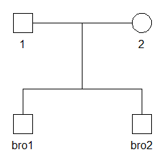
We start by creating and plotting a pedigree with two brothers, named bro1 and bro2.

x = nuclearPed(children = c("bro1", "bro2"))
plot(x)

Marker simulation

Now let us simulate the genotypes of 100 independent SNPs for all four family members. Each SNP has alleles 1 and 2, with equal frequencies by default. This is an example of unconditional simulation, since we don’t give any genotypes to condition on.

x = markerSim(x, N = 100, alleles = 1:2, seed = 1234)
#> Unconditional simulation of 100 autosomal markers.
#> Individuals: 1, 2, bro1, bro2
#> Allele frequencies:
#>    1   2
#>  0.5 0.5
#> Mutation model: No 
#> 
#> Simulation finished.
#> Calls to `likelihood()`: 0.
#> Total time used: 0.02 seconds.

Note 1: The seed argument is passed onto the random number generator. If you use the same seed, you should get exactly the same results.
Note 2: To suppress the informative messages printed during simulation, add verbose = FALSE to the function call.

The pedigree x now has 100 markers attached to it. The genotypes of the first few markers are shown when printing x to the screen:

x
#>    id fid mid sex <1> <2> <3> <4> <5>
#>     1   *   *   1 1/2 1/2 1/1 2/2 2/2
#>     2   *   *   2 1/1 1/2 1/1 1/1 2/2
#>  bro1   1   2   1 1/1 1/2 1/1 1/2 2/2
#>  bro2   1   2   1 1/1 1/2 1/1 1/2 2/2
#> Only 5 (out of 100) markers are shown.

Conditional simulation

Suppose one of the brothers is homozygous 1/1 and that we want to simulate genotypes for the other brother. This is achieved with the following code, where after first attaching a marker to the pedigree, specifying the known genotype, we condition on it by referencing it in markerSim().

y = nuclearPed(children = c("bro1", "bro2")) |> 
  addMarker(bro1 = "1/1", alleles = 1:2, name = "snp1") |> 
  markerSim(N = 100, ids = "bro2", partialmarker = "snp1", 
            seed = 321, verbose = FALSE)
y
#>    id fid mid sex <1> <2> <3> <4> <5>
#>     1   *   *   1 -/- -/- -/- -/- -/-
#>     2   *   *   2 -/- -/- -/- -/- -/-
#>  bro1   1   2   1 1/1 1/1 1/1 1/1 1/1
#>  bro2   1   2   1 2/2 1/2 1/1 1/1 1/1
#> Only 5 (out of 100) markers are shown.

Note that the previous code also demonstrates how pedsuite is well adapted to the R pipe |>.

Estimation of IBD coefficients

The ibdEstimate() function estimates the coefficients of identity-by-descent (IBD) between pairs of individuals, from the available marker data. Let us try with the simulated genotypes we just generated:

k = ibdEstimate(y, ids = c("bro1", "bro2"))
#> Estimating 'kappa' coefficients
#> Initial search value: (0.333, 0.333, 0.333)
#> Pairs of individuals: 1
#>   bro1 vs. bro2: estimate = (0.28, 0.54, 0.18), iterations = 10
#> Total time: 0.00339 secs
k
#>    id1  id2   N      k0      k1      k2
#> 1 bro1 bro2 100 0.28001 0.53998 0.18001

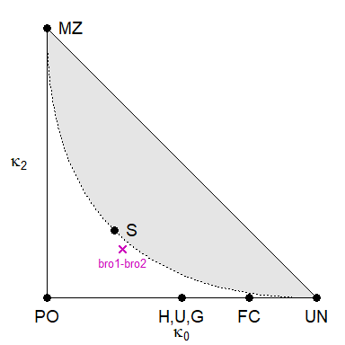
To get a visual sense of the estimate, it is instructive to plot it in the IBD triangle:

showInTriangle(k, labels = TRUE)

Reassuringly, the estimate is close to the theoretical expectation for non-inbred full siblings, \((\kappa_0, \kappa_1, \kappa_2) = (0.25, 0.5, 0.25)\), corresponding to the point marked S in the triangle.

These binaries (installable software) and packages are in development.
They may not be fully stable and should be used with caution. We make no claims about them.