The hardware and bandwidth for this mirror is donated by METANET, the Webhosting and Full Service-Cloud Provider.
If you wish to report a bug, or if you are interested in having us mirror your free-software or open-source project, please feel free to contact us at mirror[@]metanet.ch.







An R package for fitting and testing specifications of fractional regression models. It handles fractional, univariate proportions, and bounded data (\(0 \le y \le 1\)), and provides estimators for one-part, two-part (hurdle), and three-part (double-inflated) models. It also extends fractional modelling to multivariate data through fractional multinomial logit and introduces fractional ridge regression for multicollinear, high-dimensional datasets.
fracreg handles:
fracreg): Fit standard 1-part models, hurdle
2-part models (mass at 0 or 1), and double-inflated 3-part models.fracregpd):
Estimate fractional models with fixed-T longitudinal data, supporting
Correlated Random Effects (CRE) to handle unobserved individual
heterogeneity.fracreghet): Correct for endogenous covariates
using Instrumental Variables (IV) via Control Function and GMM
approaches.fracregmlogit): Estimate multivariate fractional
responses where outcomes across multiple categories sum to 1.fracregridge): Perform L2 regularization using
dynamic fraction penalties of the unregularized vector length.fracreg.ggoff,
fracreghet.reset, fracreg.ptest).fracreg.pe(), fracregpd.pe(),
fracreghet.pe(), fracregridge.pe(), and
fracregmlogit.pe()).coef(), predict(),
fitted(), residuals(), vcov(),
logLik(), nobs()) and native
na.action missing data handling across all estimators.You can install the released version of fracreg from
CRAN with:
install.packages("fracreg")
library("fracreg")
Or install the development version from GitHub:
# install.packages("devtools")
devtools::install_github("SulmanOlieko/fracreg")This guide walks you through comprehensive empirical examples (using the 401(k) dataset) and simulated examples for each estimator.
We use the built-in fracreg_k401k dataset, which is the
canonical firm-level 401(k) plan participation data used in
Papke and Wooldridge (1996) (“Econometric methods
for fractional response variables with an application to 401(k) plan
participation rates”, Journal of Applied Econometrics). The dataset
contains 1,534 observations of 401(k) plans.
The primary variables we use are: - prate: The plan
participation rate (the fraction of eligible employees who are active
participants). It strictly falls in the \([0,
1]\) interval and is our dependent variable (\(y\)). - mrate: The firm’s
matching rate (the firm’s contribution per $1 of employee contribution).
- age: The age of the 401(k) plan. - totemp:
Total number of employees at the firm. - sole: A binary
indicator equal to 1 if the 401(k) plan is the sole retirement plan
offered by the firm.
fracreg)The core fracreg() function is designed for univariate
models where the dependent variable is bounded between 0 and 1 inclusive
(\(0 \le y \le 1\)). The examples below
demonstrate both empirical 401(k) plan participation data and general
simulated boundaries.
### Empirical 401(k) Examples
data("fracreg_k401k")
y <- fracreg_k401k$prate
X <- cbind(mrate = fracreg_k401k$mrate, age = fracreg_k401k$age,
           totemp = fracreg_k401k$totemp, sole = fracreg_k401k$sole)

# 1P Model
mod <- fracreg(y, X, type="1P", linkfrac="logit")
summary(mod)#>
#> --------------------------------------------------------------------------------
#> Fractional logit regression
#> --------------------------------------------------------------------------------
#> Data type: Cross-sectional
#> Estimator: QML
#> Convergence: Successful
#> Number of observations: 1534
#> Log pseudolikelihood: -553.1626
#> Pseudo R-squared: 0.14667
#> Wald chi2(4): 147.3049
#> Prob > chi2: 0.0000
#> Standard errors: HC0
#> Small sample correction: FALSE
#> --------------------------------------------------------------------------------
#> Final Quasi-Maximum Likelihood estimates
#> --------------------------------------------------------------------------------
#> Coefficient Robust Std.Err. z value [95% Conf. Interval]
#> (Intercept) 9.316e-01 8.408e-02 1.108e+01 7.668e-01 1.096
#> mrate 9.531e-01 1.371e-01 6.951e+00 6.843e-01 1.222
#> age 2.791e-02 4.877e-03 5.723e+00 1.835e-02 0.037
#> totemp -8.182e-06 3.061e-06 -2.673e+00 -1.418e-05 0.000
#> sole 3.405e-01 8.066e-02 4.222e+00 1.824e-01 0.499
#> Pr(>|z|)
#> (Intercept) < 2e-16 ***
#> mrate 3.62e-12 ***
#> age 1.05e-08 ***
#> totemp 0.00751 **
#> sole 2.43e-05 ***
#> ---
#> Signif. codes: 0 '***' 0.001 '**' 0.01 '*' 0.05 '.' 0.1 ' ' 1
#> --------------------------------------------------------------------------------
#> Run Date: 2026-08-08 17:44:22
#> --------------------------------------------------------------------------------
# 1P Model reporting odds ratios and 99% confidence intervals
mod <- fracreg(y, X, type="1P", linkfrac="logit", or=TRUE, level=0.99)
summary(mod)#>
#> --------------------------------------------------------------------------------
#> Fractional logit regression
#> --------------------------------------------------------------------------------
#> Data type: Cross-sectional
#> Estimator: QML
#> Convergence: Successful
#> Number of observations: 1534
#> Log pseudolikelihood: -553.1626
#> Pseudo R-squared: 0.14667
#> Wald chi2(4): 147.3049
#> Prob > chi2: 0.0000
#> Standard errors: HC0
#> Small sample correction: FALSE
#> --------------------------------------------------------------------------------
#> Final Quasi-Maximum Likelihood estimates
#> --------------------------------------------------------------------------------
#> Odds Ratio Robust Std.Err. z value [99% Conf. Interval] Pr(>|z|)
#> (Intercept) 2.539e+00 2.134e-01 1.108e+01 2.044e+00 3.153 < 2e-16
#> mrate 2.594e+00 3.556e-01 6.951e+00 1.822e+00 3.692 3.62e-12
#> age 1.028e+00 5.015e-03 5.723e+00 1.015e+00 1.041 1.05e-08
#> totemp 1.000e+00 3.061e-06 -2.673e+00 1.000e+00 1.000 0.00751
#> sole 1.406e+00 1.134e-01 4.222e+00 1.142e+00 1.730 2.43e-05
#>
#> (Intercept) ***
#> mrate ***
#> age ***
#> totemp **
#> sole ***
#> ---
#> Signif. codes: 0 '***' 0.001 '**' 0.01 '*' 0.05 '.' 0.1 ' ' 1
#> --------------------------------------------------------------------------------
#> Run Date: 2026-08-08 17:44:23
#> --------------------------------------------------------------------------------
# 2P Model (modelling mass at 1)
mod <- fracreg(y, X, type="2P", inflation=1, linkbin="logit", linkfrac="logit")
summary(mod)#>
#> --------------------------------------------------------------------------------
#> Part 1: Binary logit regression
#> --------------------------------------------------------------------------------
#> Data type: Cross-sectional
#> Estimator: ML
#> Convergence: Successful
#> Number of observations: 1534
#> Log-likelihood: -938.1759
#> Pseudo R-squared: 0.1485
#> Wald chi2(4): 173.5169
#> Prob > chi2: 0.0000
#> Small sample correction: FALSE
#> --------------------------------------------------------------------------------
#> Final Maximum Likelihood estimates
#> --------------------------------------------------------------------------------
#> Coefficient EIM Std.Err. z value [95% Conf. Interval] Pr(>|z|)
#> (Intercept) -1.396e+00 1.270e-01 -1.099e+01 -1.645e+00 -1.147 <2e-16
#> mrate 9.053e-01 9.699e-02 9.334e+00 7.152e-01 1.095 <2e-16
#> age 1.156e-02 6.218e-03 1.858e+00 -6.312e-04 0.024 0.0631
#> totemp -1.418e-05 6.324e-06 -2.242e+00 -2.657e-05 0.000 0.0249
#> sole 8.651e-01 1.131e-01 7.651e+00 6.435e-01 1.087 2e-14
#>
#> (Intercept) ***
#> mrate ***
#> age .
#> totemp *
#> sole ***
#> ---
#> Signif. codes: 0 '***' 0.001 '**' 0.01 '*' 0.05 '.' 0.1 ' ' 1
#> --------------------------------------------------------------------------------
#>
#>
#> --------------------------------------------------------------------------------
#> Part 2: Fractional logit regression
#> --------------------------------------------------------------------------------
#> Data type: Cross-sectional
#> Estimator: QML
#> Convergence: Successful
#> Number of observations: 852
#> Log pseudolikelihood: -450.8391
#> Pseudo R-squared: 0.10004
#> Wald chi2(4): 65.4063
#> Prob > chi2: 0.0000
#> Standard errors: HC0
#> Small sample correction: FALSE
#> --------------------------------------------------------------------------------
#> Final Quasi-Maximum Likelihood estimates
#> --------------------------------------------------------------------------------
#> Coefficient Robust Std.Err. z value [95% Conf. Interval]
#> (Intercept) 7.460e-01 6.850e-02 1.089e+01 6.118e-01 0.880
#> mrate 3.877e-01 9.725e-02 3.987e+00 1.971e-01 0.578
#> age 2.562e-02 4.010e-03 6.390e+00 1.777e-02 0.033
#> totemp -4.061e-06 3.073e-06 -1.322e+00 -1.008e-05 0.000
#> sole -1.510e-02 6.556e-02 -2.303e-01 -1.436e-01 0.113
#> Pr(>|z|)
#> (Intercept) < 2e-16 ***
#> mrate 6.69e-05 ***
#> age 1.66e-10 ***
#> totemp 0.186
#> sole 0.818
#> ---
#> Signif. codes: 0 '***' 0.001 '**' 0.01 '*' 0.05 '.' 0.1 ' ' 1
#> --------------------------------------------------------------------------------
#>
#>
#> --------------------------------------------------------------------------------
#> Two-part fractional regression: binary logit + fractional logit
#> --------------------------------------------------------------------------------
#> Data type: Cross-sectional
#> Convergence: Successful
#> Pseudo R-squared: 0.11243
#> --------------------------------------------------------------------------------
#> Run Date: 2026-08-08 17:44:23
#> --------------------------------------------------------------------------------
# 3P Model (inject artificial 0s for demonstration)
y_3p <- y; y_3p[1:50] <- 0
mod <- fracreg(y_3p, X, type="3P", linkbin=c("logit","logit"), linkfrac="logit")
summary(mod)#>
#> --------------------------------------------------------------------------------
#> Part 1: Binary logit regression
#> --------------------------------------------------------------------------------
#> Data type: Cross-sectional
#> Estimator: ML
#> Convergence: Successful
#> Number of observations: 1534
#> Log-likelihood: -216.6222
#> Pseudo R-squared: 0.00324
#> Wald chi2(4): 3.7679
#> Prob > chi2: 0.4383
#> Small sample correction: FALSE
#> --------------------------------------------------------------------------------
#> Final Maximum Likelihood estimates
#> --------------------------------------------------------------------------------
#> Coefficient EIM Std.Err. z value [95% Conf. Interval] Pr(>|z|)
#> (Intercept) 2.867e+00 3.157e-01 9.080e+00 2.248e+00 3.486 <2e-16
#> mrate 1.147e-01 2.131e-01 5.381e-01 -3.030e-01 0.532 0.590
#> age 8.375e-03 1.765e-02 4.745e-01 -2.622e-02 0.043 0.635
#> totemp 1.036e-04 6.959e-05 1.489e+00 -3.275e-05 0.000 0.136
#> sole 3.371e-01 2.983e-01 1.130e+00 -2.476e-01 0.922 0.259
#>
#> (Intercept) ***
#> mrate
#> age
#> totemp
#> sole
#> ---
#> Signif. codes: 0 '***' 0.001 '**' 0.01 '*' 0.05 '.' 0.1 ' ' 1
#> --------------------------------------------------------------------------------
#>
#>
#> --------------------------------------------------------------------------------
#> Part 2: Binary logit regression
#> --------------------------------------------------------------------------------
#> Data type: Cross-sectional
#> Estimator: ML
#> Convergence: Successful
#> Number of observations: 1484
#> Log-likelihood: -903.5457
#> Pseudo R-squared: 0.15199
#> Wald chi2(4): 172.201
#> Prob > chi2: 0.0000
#> Small sample correction: FALSE
#> --------------------------------------------------------------------------------
#> Final Maximum Likelihood estimates
#> --------------------------------------------------------------------------------
#> Coefficient EIM Std.Err. z value [95% Conf. Interval] Pr(>|z|)
#> (Intercept) -1.435e+00 1.306e-01 -1.099e+01 -1.691e+00 -1.179 < 2e-16
#> mrate 9.244e-01 9.877e-02 9.360e+00 7.309e-01 1.118 < 2e-16
#> age 1.198e-02 6.339e-03 1.890e+00 -4.453e-04 0.024 0.0588
#> totemp -1.371e-05 6.317e-06 -2.170e+00 -2.609e-05 0.000 0.0300
#> sole 8.852e-01 1.154e-01 7.674e+00 6.591e-01 1.111 1.67e-14
#>
#> (Intercept) ***
#> mrate ***
#> age .
#> totemp *
#> sole ***
#> ---
#> Signif. codes: 0 '***' 0.001 '**' 0.01 '*' 0.05 '.' 0.1 ' ' 1
#> --------------------------------------------------------------------------------
#>
#>
#> --------------------------------------------------------------------------------
#> Part 3: Fractional logit regression
#> --------------------------------------------------------------------------------
#> Data type: Cross-sectional
#> Estimator: QML
#> Convergence: Successful
#> Number of observations: 826
#> Log pseudolikelihood: -437.3715
#> Pseudo R-squared: 0.09937
#> Wald chi2(4): 62.3685
#> Prob > chi2: 0.0000
#> Standard errors: HC0
#> Small sample correction: FALSE
#> --------------------------------------------------------------------------------
#> Final Quasi-Maximum Likelihood estimates
#> --------------------------------------------------------------------------------
#> Coefficient Robust Std.Err. z value [95% Conf. Interval]
#> (Intercept) 7.388e-01 7.039e-02 1.050e+01 6.008e-01 0.877
#> mrate 3.960e-01 1.019e-01 3.885e+00 1.962e-01 0.596
#> age 2.531e-02 4.068e-03 6.223e+00 1.734e-02 0.033
#> totemp -3.817e-06 3.088e-06 -1.236e+00 -9.869e-06 0.000
#> sole -4.483e-03 6.672e-02 -6.719e-02 -1.353e-01 0.126
#> Pr(>|z|)
#> (Intercept) < 2e-16 ***
#> mrate 0.000102 ***
#> age 4.88e-10 ***
#> totemp 0.216472
#> sole 0.946434
#> ---
#> Signif. codes: 0 '***' 0.001 '**' 0.01 '*' 0.05 '.' 0.1 ' ' 1
#> --------------------------------------------------------------------------------
#>
#>
#> --------------------------------------------------------------------------------
#> Three-part fractional regression: binary logit , binary logit + fractional logit
#> --------------------------------------------------------------------------------
#> Data type: Cross-sectional
#> Convergence: Successful
#> Pseudo R-squared: 0.07934
#> --------------------------------------------------------------------------------
#> Run Date: 2026-08-08 17:44:23
#> --------------------------------------------------------------------------------
### Simulated Examples

set.seed(123)
N <- 1000
x1 <- rnorm(N)
x2 <- runif(N)

# Generating a fractional dependent variable with inflation at 0 and 1
XB <- -0.5 + 0.8 * x1 + 1.2 * x2 + rnorm(N)
y_latent <- exp(XB) / (1 + exp(XB))

y <- y_latent
# Inflate at boundaries
y[y_latent < 0.2] <- 0
y[y_latent > 0.8] <- 1

X <- cbind(x1 = x1, x2 = x2)

# fracreg estimation of a logit fractional response model
mod <- fracreg(y, X, type="1P", linkfrac="logit")
summary(mod)#>
#> --------------------------------------------------------------------------------
#> Fractional logit regression
#> --------------------------------------------------------------------------------
#> Data type: Cross-sectional
#> Estimator: QML
#> Convergence: Successful
#> Number of observations: 1000
#> Log pseudolikelihood: -614.973
#> Pseudo R-squared: 0.3903
#> Wald chi2(2): 472.2453
#> Prob > chi2: 0.0000
#> Standard errors: HC0
#> Small sample correction: FALSE
#> --------------------------------------------------------------------------------
#> Final Quasi-Maximum Likelihood estimates
#> --------------------------------------------------------------------------------
#> Coefficient Robust Std.Err. z value [95% Conf. Interval] Pr(>|z|)
#> (Intercept) -0.56969 0.06750 -8.43960 -0.70199 -0.437 <2e-16
#> x1 0.78822 0.04015 19.63424 0.70954 0.867 <2e-16
#> x2 1.35611 0.11899 11.39668 1.12289 1.589 <2e-16
#>
#> (Intercept) ***
#> x1 ***
#> x2 ***
#> ---
#> Signif. codes: 0 '***' 0.001 '**' 0.01 '*' 0.05 '.' 0.1 ' ' 1
#> --------------------------------------------------------------------------------
#> Run Date: 2026-08-08 17:44:23
#> --------------------------------------------------------------------------------
# fracreg estimation of the binary logit component of the two-part fractional
# regression model with y=0 as the relevant boundary value
mod <- fracreg(y, X, type="2Pbin", inflation=0, linkbin="logit")
summary(mod)#>
#> --------------------------------------------------------------------------------
#> Part 1: Binary logit regression
#> --------------------------------------------------------------------------------
#> Data type: Cross-sectional
#> Estimator: ML
#> Convergence: Successful
#> Number of observations: 1000
#> Log-likelihood: -295.2068
#> Pseudo R-squared: 0.14527
#> Wald chi2(2): 102.5171
#> Prob > chi2: 0.0000
#> Small sample correction: FALSE
#> --------------------------------------------------------------------------------
#> Final Maximum Likelihood estimates
#> --------------------------------------------------------------------------------
#> Coefficient EIM Std.Err. z value [95% Conf. Interval] Pr(>|z|)
#> (Intercept) 1.4638 0.1933 7.5732 1.0849 1.843 3.64e-14 ***
#> x1 1.1857 0.1287 9.2126 0.9335 1.438 < 2e-16 ***
#> x2 2.2279 0.3932 5.6662 1.4572 2.999 1.46e-08 ***
#> ---
#> Signif. codes: 0 '***' 0.001 '**' 0.01 '*' 0.05 '.' 0.1 ' ' 1
#> --------------------------------------------------------------------------------
# fracreg estimation of the fractional component of the two-part fractional
# regression model with y=0 as the relevant boundary value and using a
# probit link function
mod <- fracreg(y, X, type="2Pfrac", inflation=0, linkfrac="probit")
summary(mod)#>
#> --------------------------------------------------------------------------------
#> Part 2: Fractional probit regression
#> --------------------------------------------------------------------------------
#> Data type: Cross-sectional
#> Estimator: QML
#> Convergence: Successful
#> Number of observations: 881
#> Log pseudolikelihood: -555.3304
#> Pseudo R-squared: 0.32474
#> Wald chi2(2): 391.6944
#> Prob > chi2: 0.0000
#> Standard errors: HC0
#> Small sample correction: FALSE
#> --------------------------------------------------------------------------------
#> Final Quasi-Maximum Likelihood estimates
#> --------------------------------------------------------------------------------
#> Coefficient Robust Std.Err. z value [95% Conf. Interval] Pr(>|z|)
#> (Intercept) -0.10334 0.03566 -2.89793 -0.17323 -0.033 0.00376
#> x1 0.37512 0.02129 17.62293 0.33340 0.417 < 2e-16
#> x2 0.61326 0.06529 9.39237 0.48529 0.741 < 2e-16
#>
#> (Intercept) **
#> x1 ***
#> x2 ***
#> ---
#> Signif. codes: 0 '***' 0.001 '**' 0.01 '*' 0.05 '.' 0.1 ' ' 1
#> --------------------------------------------------------------------------------
# fracreg estimation of both components of a two-part fractional response model
# with y=0 as the relevant boundary value and using a cloglog binary link
# function and a logit fractional link function
mod <- fracreg(y, X, type="2P", inflation=0, linkbin="cloglog", linkfrac="logit")
summary(mod)#>
#> --------------------------------------------------------------------------------
#> Part 1: Binary cloglog regression
#> --------------------------------------------------------------------------------
#> Data type: Cross-sectional
#> Estimator: ML
#> Convergence: Successful
#> Number of observations: 1000
#> Log-likelihood: -291.7986
#> Pseudo R-squared: 0.14837
#> Wald chi2(2): 100.5683
#> Prob > chi2: 0.0000
#> Small sample correction: FALSE
#> --------------------------------------------------------------------------------
#> Final Maximum Likelihood estimates
#> --------------------------------------------------------------------------------
#> Coefficient EIM Std.Err. z value [95% Conf. Interval] Pr(>|z|)
#> (Intercept) 0.43428 0.08825 4.92113 0.26132 0.607 8.60e-07 ***
#> x1 0.55192 0.06009 9.18429 0.43414 0.670 < 2e-16 ***
#> x2 1.05359 0.17403 6.05409 0.71250 1.395 1.41e-09 ***
#> ---
#> Signif. codes: 0 '***' 0.001 '**' 0.01 '*' 0.05 '.' 0.1 ' ' 1
#> --------------------------------------------------------------------------------
#>
#>
#> --------------------------------------------------------------------------------
#> Part 2: Fractional logit regression
#> --------------------------------------------------------------------------------
#> Data type: Cross-sectional
#> Estimator: QML
#> Convergence: Successful
#> Number of observations: 881
#> Log pseudolikelihood: -555.4465
#> Pseudo R-squared: 0.32412
#> Wald chi2(2): 368.0384
#> Prob > chi2: 0.0000
#> Standard errors: HC0
#> Small sample correction: FALSE
#> --------------------------------------------------------------------------------
#> Final Quasi-Maximum Likelihood estimates
#> --------------------------------------------------------------------------------
#> Coefficient Robust Std.Err. z value [95% Conf. Interval] Pr(>|z|)
#> (Intercept) -0.17323 0.05786 -2.99384 -0.28664 -0.060 0.00275
#> x1 0.61205 0.03554 17.22078 0.54239 0.682 < 2e-16
#> x2 1.00509 0.10703 9.39074 0.79531 1.215 < 2e-16
#>
#> (Intercept) **
#> x1 ***
#> x2 ***
#> ---
#> Signif. codes: 0 '***' 0.001 '**' 0.01 '*' 0.05 '.' 0.1 ' ' 1
#> --------------------------------------------------------------------------------
#>
#>
#> --------------------------------------------------------------------------------
#> Two-part fractional regression: binary cloglog + fractional logit
#> --------------------------------------------------------------------------------
#> Data type: Cross-sectional
#> Convergence: Successful
#> Pseudo R-squared: 0.38829
#> --------------------------------------------------------------------------------
#> Run Date: 2026-08-08 17:44:24
#> --------------------------------------------------------------------------------
# Three-part double-inflated model (y has both 0s and 1s)
mod <- fracreg(y, X, type="3P", linkbin=c("logit","probit"), linkfrac="logit")
summary(mod)#>
#> --------------------------------------------------------------------------------
#> Part 1: Binary logit regression
#> --------------------------------------------------------------------------------
#> Data type: Cross-sectional
#> Estimator: ML
#> Convergence: Successful
#> Number of observations: 1000
#> Log-likelihood: -295.2068
#> Pseudo R-squared: 0.14527
#> Wald chi2(2): 102.5171
#> Prob > chi2: 0.0000
#> Small sample correction: FALSE
#> --------------------------------------------------------------------------------
#> Final Maximum Likelihood estimates
#> --------------------------------------------------------------------------------
#> Coefficient EIM Std.Err. z value [95% Conf. Interval] Pr(>|z|)
#> (Intercept) 1.4638 0.1933 7.5732 1.0849 1.843 3.64e-14 ***
#> x1 1.1857 0.1287 9.2126 0.9335 1.438 < 2e-16 ***
#> x2 2.2279 0.3932 5.6662 1.4572 2.999 1.46e-08 ***
#> ---
#> Signif. codes: 0 '***' 0.001 '**' 0.01 '*' 0.05 '.' 0.1 ' ' 1
#> --------------------------------------------------------------------------------
#>
#>
#> --------------------------------------------------------------------------------
#> Part 2: Binary probit regression
#> --------------------------------------------------------------------------------
#> Data type: Cross-sectional
#> Estimator: ML
#> Convergence: Successful
#> Number of observations: 881
#> Log-likelihood: -348.8644
#> Pseudo R-squared: 0.18634
#> Wald chi2(2): 123.5731
#> Prob > chi2: 0.0000
#> Small sample correction: FALSE
#> --------------------------------------------------------------------------------
#> Final Maximum Likelihood estimates
#> --------------------------------------------------------------------------------
#> Coefficient EIM Std.Err. z value [95% Conf. Interval] Pr(>|z|)
#> (Intercept) -1.71537 0.12933 -13.26354 -1.96885 -1.462 < 2e-16
#> x1 0.64810 0.06323 10.25024 0.52418 0.772 < 2e-16
#> x2 1.07752 0.19174 5.61978 0.70172 1.453 1.91e-08
#>
#> (Intercept) ***
#> x1 ***
#> x2 ***
#> ---
#> Signif. codes: 0 '***' 0.001 '**' 0.01 '*' 0.05 '.' 0.1 ' ' 1
#> --------------------------------------------------------------------------------
#>
#>
#> --------------------------------------------------------------------------------
#> Part 3: Fractional logit regression
#> --------------------------------------------------------------------------------
#> Data type: Cross-sectional
#> Estimator: QML
#> Convergence: Successful
#> Number of observations: 715
#> Log pseudolikelihood: -484.9654
#> Pseudo R-squared: 0.24292
#> Wald chi2(2): 261.436
#> Prob > chi2: 0.0000
#> Standard errors: HC0
#> Small sample correction: FALSE
#> --------------------------------------------------------------------------------
#> Final Quasi-Maximum Likelihood estimates
#> --------------------------------------------------------------------------------
#> Coefficient Robust Std.Err. z value [95% Conf. Interval] Pr(>|z|)
#> (Intercept) -0.26763 0.04539 -5.89578 -0.35660 -0.179 3.73e-09
#> x1 0.36198 0.02454 14.75144 0.31389 0.410 < 2e-16
#> x2 0.58505 0.07969 7.34179 0.42886 0.741 2.11e-13
#>
#> (Intercept) ***
#> x1 ***
#> x2 ***
#> ---
#> Signif. codes: 0 '***' 0.001 '**' 0.01 '*' 0.05 '.' 0.1 ' ' 1
#> --------------------------------------------------------------------------------
#>
#>
#> --------------------------------------------------------------------------------
#> Three-part fractional regression: binary logit , binary probit + fractional logit
#> --------------------------------------------------------------------------------
#> Data type: Cross-sectional
#> Convergence: Successful
#> Pseudo R-squared: 0.38917
#> --------------------------------------------------------------------------------
#> Run Date: 2026-08-08 17:44:24
#> --------------------------------------------------------------------------------fracreg.pe)Raw coefficients from fractional models are not directly
interpretable as marginal effects. Use fracreg.pe() to
compute the Average Partial Effects (APE) and Conditional Partial
Effects (CPE) using the analytical delta method.
### Empirical 401(k) Examples
data("fracreg_k401k")
y <- fracreg_k401k$prate
X <- cbind(mrate = fracreg_k401k$mrate, age = fracreg_k401k$age,
           totemp = fracreg_k401k$totemp, sole = fracreg_k401k$sole)

m <- fracreg(y, X, type="1P", linkfrac="logit")
pe_res <- fracreg.pe(m)
summary(pe_res)#>
#> --------------------------------------------------------------------------------
#> Average partial effects
#> --------------------------------------------------------------------------------
#> Fractional logit regression
#> --------------------------------------------------------------------------------
#>
#> Note: Standard errors computed using the Delta method
#> dy/dx Std. Error z value Pr(>|z|)
#> mrate 1.018e-01 1.456e-02 6.989 2.77e-12 ***
#> age 2.980e-03 5.293e-04 5.630 1.80e-08 ***
#> totemp -8.736e-07 3.279e-07 -2.665 0.00771 **
#> sole 3.635e-02 8.515e-03 4.270 1.96e-05 ***
#> ---
#> Signif. codes: 0 '***' 0.001 '**' 0.01 '*' 0.05 '.' 0.1 ' ' 1
#> --------------------------------------------------------------------------------
#> Run Date: 2026-08-08 17:44:24
#> --------------------------------------------------------------------------------
### Simulated Examples

N <- 250
u <- rnorm(N)

X <- cbind(rnorm(N),rnorm(N))
dimnames(X)[[2]] <- c("X1","X2")

ym <- exp(X[,1]+X[,2]+u)/(1+exp(X[,1]+X[,2]+u))
y <- rbeta(N,ym*20,20*(1-ym))
y[y > 0.9] <- 1

#Computing average partial effects for a logit fractional response model
mod <- fracreg(y,X,linkfrac="logit")
pe_res <- fracreg.pe(mod)
summary(pe_res)#>
#> --------------------------------------------------------------------------------
#> Average partial effects
#> --------------------------------------------------------------------------------
#> Fractional logit regression
#> --------------------------------------------------------------------------------
#>
#> Note: Standard errors computed using the Delta method
#> dy/dx Std. Error z value Pr(>|z|)
#> X1 0.161653 0.009584 16.87 <2e-16 ***
#> X2 0.165141 0.012853 12.85 <2e-16 ***
#> ---
#> Signif. codes: 0 '***' 0.001 '**' 0.01 '*' 0.05 '.' 0.1 ' ' 1
#> --------------------------------------------------------------------------------
#> Run Date: 2026-08-08 17:44:25
#> --------------------------------------------------------------------------------
#Computing average partial effects for a binary logit + fractional probit
#two-part model
mod <- fracreg(y,X,linkbin="logit",linkfrac="probit",type="2P",inf=1)
pe_res <- fracreg.pe(mod)
summary(pe_res)#>
#>
#> --------------------------------------------------------------------------------
#> Average partial effects
#> --------------------------------------------------------------------------------
#>
#> Binary logit regression (Pr(y = 1)):
#>
#> Note: Standard errors computed using the Delta method
#> dy/dx Std. Error z value Pr(>|z|)
#> X1 0.10163 0.01549 6.560 5.37e-11 ***
#> X2 0.10992 0.01649 6.665 2.64e-11 ***
#>
#> Fractional probit regression (Fractional Component):
#>
#> Note: Standard errors computed using the Delta method
#> dy/dx Std. Error z value Pr(>|z|)
#> X1 0.14809 0.01068 13.86 <2e-16 ***
#> X2 0.14840 0.01407 10.55 <2e-16 ***
#>
#> --------------------------------------------------------------------------------
#> Binary logit + Fractional probit two-part regression
#> --------------------------------------------------------------------------------
#>
#> Note: Standard errors computed using the Delta method
#> dy/dx Std. Error z value Pr(>|z|)
#> X1 0.08479 0.01192 7.115 1.12e-12 ***
#> X2 0.09068 0.01249 7.259 3.89e-13 ***
#> ---
#> Signif. codes: 0 '***' 0.001 '**' 0.01 '*' 0.05 '.' 0.1 ' ' 1
#> --------------------------------------------------------------------------------
#> Run Date: 2026-08-08 17:44:25
#> --------------------------------------------------------------------------------
#Computing conditional partial effects for X2 in the logit component
#of a two-part fractional response model, with the covariates evaluated
#at their median values
mod <- fracreg(y,X,linkfrac="logit",type="2Pfrac",inf=1)
pe_res <- fracreg.pe(mod,APE=FALSE,CPE=TRUE,at="median",which.x="X2")
summary(pe_res)#>
#> --------------------------------------------------------------------------------
#> Conditional partial effects
#> --------------------------------------------------------------------------------
#> Fractional logit component of a two-part regression
#> --------------------------------------------------------------------------------
#>
#> Note: Standard errors computed using the Delta method
#> dy/dx Std. Error z value Pr(>|z|)
#> X2 0.17106 0.01895 9.026 <2e-16 ***
#> ---
#> Signif. codes: 0 '***' 0.001 '**' 0.01 '*' 0.05 '.' 0.1 ' ' 1
#> --------------------------------------------------------------------------------
#> Run Date: 2026-08-08 17:44:25
#> --------------------------------------------------------------------------------
#>
#> Note: covariates evaluated at median (or mode, for dummies) values
#Computing average partial effects for a three-part double-inflated model
y3p <- y
y3p[1:20] <- 0
y3p[21:40] <- 1
res3p <- fracreg(y3p,X,linkbin=c("logit","probit"),linkfrac="logit",type="3P")
pe_res <- fracreg.pe(res3p)
summary(pe_res)#>
#>
#> --------------------------------------------------------------------------------
#> Average partial effects
#> --------------------------------------------------------------------------------
#>
#> Binary logit regression (Pr(y > 0)):
#>
#> Note: Standard errors computed using the Delta method
#> dy/dx Std. Error z value Pr(>|z|)
#> X1 0.006772 0.016605 0.408 0.683
#> X2 -0.020995 0.017401 -1.207 0.228
#>
#> Binary probit regression (Pr(y = 1 | y > 0)):
#>
#> Note: Standard errors computed using the Delta method
#> dy/dx Std. Error z value Pr(>|z|)
#> X1 0.11296 0.02152 5.249 1.53e-07 ***
#> X2 0.06011 0.02444 2.460 0.0139 *
#>
#> Fractional logit regression (Fractional Component):
#>
#> Note: Standard errors computed using the Delta method
#> dy/dx Std. Error z value Pr(>|z|)
#> X1 0.14591 0.01227 11.893 <2e-16 ***
#> X2 0.14019 0.01645 8.521 <2e-16 ***
#>
#> --------------------------------------------------------------------------------
#> Three-part regression - binary logit , binary probit + fractional logit
#> --------------------------------------------------------------------------------
#>
#> Note: Standard errors computed using the Delta method
#> dy/dx Std. Error z value Pr(>|z|)
#> X1 0.15535 0.01440 10.790 < 2e-16 ***
#> X2 0.11405 0.01854 6.153 7.62e-10 ***
#> ---
#> Signif. codes: 0 '***' 0.001 '**' 0.01 '*' 0.05 '.' 0.1 ' ' 1
#> --------------------------------------------------------------------------------
#> Run Date: 2026-08-08 17:44:25
#> --------------------------------------------------------------------------------fracreg includes state-of-the-art specification tests to
validate your model’s functional form and link function assumptions.
fracreg.ggoff)The GGOFF test tests whether the chosen link function is adequate for the data. A significant result suggests the link may be misspecified.
### Empirical 401(k) Examples
data("fracreg_k401k")
y <- fracreg_k401k$prate
X <- cbind(mrate = fracreg_k401k$mrate, age = fracreg_k401k$age,
           totemp = fracreg_k401k$totemp, sole = fracreg_k401k$sole)

m <- fracreg(y, X, type="1P", linkfrac="logit")
ggoff_res <- fracreg.ggoff(m)
summary(ggoff_res)#>
#> --------------------------------------------------------------------------------
#> GGOFF test
#> --------------------------------------------------------------------------------
#> H0: Fractional logit regression
#> --------------------------------------------------------------------------------
#> Statistic p-value
#> GOFF1 - LM 8.838 0.00295 **
#> GOFF2 - LM 9.828 0.00172 **
#> GGOFF - LM 10.351 0.00565 **
#> ---
#> Signif. codes: 0 '***' 0.001 '**' 0.01 '*' 0.05 '.' 0.1 ' ' 1
#> --------------------------------------------------------------------------------
#> Run Date: 2026-08-08 17:44:25
#> --------------------------------------------------------------------------------
### Simulated Examples

N <- 250
u <- rnorm(N)

X <- cbind(rnorm(N),rnorm(N))
dimnames(X)[[2]] <- c("X1","X2")

ym <- exp(X[,1]+X[,2]+u)/(1+exp(X[,1]+X[,2]+u))
y <- rbeta(N,ym*20,20*(1-ym))
y[y > 0.9] <- 1

#Testing the logit specification of a standard fractional response model
#using LM and Wald versions of the GGOFF test, based on 1 or 2 fitted powers of
#the linear predictor
mod <- fracreg(y,X,linkfrac="logit")
ggoff_res <- fracreg.ggoff(mod,c("Wald","LM"))
summary(ggoff_res)#>
#> --------------------------------------------------------------------------------
#> GGOFF test
#> --------------------------------------------------------------------------------
#> H0: Fractional logit regression
#> --------------------------------------------------------------------------------
#> Statistic p-value
#> GOFF1 - LM 1.256 0.262
#> GOFF1 - Wald 1.274 0.259
#> GOFF2 - LM 1.513 0.219
#> GOFF2 - Wald 1.401 0.237
#> GGOFF - LM 1.612 0.447
#> GGOFF - Wald 1.336 0.513
#> --------------------------------------------------------------------------------
#> Run Date: 2026-08-08 17:44:25
#> --------------------------------------------------------------------------------
#Testing the probit specification of the binary component of a two-part fractional
#regression model using a LR-based GGOFF test
mod <- fracreg(y,X,linkbin="probit",type="2Pbin",inf=1)
ggoff_res <- fracreg.ggoff(mod,"LR")
summary(ggoff_res)#>
#> --------------------------------------------------------------------------------
#> GGOFF test
#> --------------------------------------------------------------------------------
#> H0: Binary probit component of a two-part regression
#> --------------------------------------------------------------------------------
#> Statistic p-value
#> GOFF1 - LR 0.012 0.914
#> GOFF2 - LR 0.017 0.895
#> GGOFF - LR 0.024 0.988
#> --------------------------------------------------------------------------------
#> Run Date: 2026-08-08 17:44:25
#> --------------------------------------------------------------------------------fracreg.reset)The RESET test detects general functional form misspecification by testing whether powers of the fitted values have explanatory power. Testing \(H_0: \gamma = 0\) provides a robust diagnostic check.
### Empirical 401(k) Examples
data("fracreg_k401k")
y <- fracreg_k401k$prate
X <- cbind(mrate = fracreg_k401k$mrate, age = fracreg_k401k$age,
           totemp = fracreg_k401k$totemp, sole = fracreg_k401k$sole)

m <- fracreg(y, X, type="1P", linkfrac="logit")
reset_res <- fracreg.reset(m)
summary(reset_res)#>
#> --------------------------------------------------------------------------------
#> RESET test
#> --------------------------------------------------------------------------------
#> H0: Fractional logit regression
#> --------------------------------------------------------------------------------
#> Statistic p-value
#> LM(3) 10.29 0.00583 **
#> ---
#> Signif. codes: 0 '***' 0.001 '**' 0.01 '*' 0.05 '.' 0.1 ' ' 1
#> --------------------------------------------------------------------------------
#> Run Date: 2026-08-08 17:44:25
#> --------------------------------------------------------------------------------
### Simulated Examples

N <- 250
u <- rnorm(N)

X <- cbind(rnorm(N),rnorm(N))
dimnames(X)[[2]] <- c("X1","X2")

ym <- exp(X[,1]+X[,2]+u)/(1+exp(X[,1]+X[,2]+u))
y <- rbeta(N,ym*20,20*(1-ym))
y[y > 0.9] <- 1

#Testing the logit specification of a standard fractional response model
#using LM and Wald versions of the RESET test, based on 1 or 2 fitted powers of
#the linear predictor
mod <- fracreg(y,X,linkfrac="logit")
reset_res <- fracreg.reset(mod,2:3,c("Wald","LM"))
summary(reset_res)#>
#> --------------------------------------------------------------------------------
#> RESET test
#> --------------------------------------------------------------------------------
#> H0: Fractional logit regression
#> --------------------------------------------------------------------------------
#> Statistic p-value
#> LM(2) 4.832 0.0279 *
#> Wald(2) 5.816 0.0159 *
#> LM(3) 4.866 0.0878 .
#> Wald(3) 6.870 0.0322 *
#> ---
#> Signif. codes: 0 '***' 0.001 '**' 0.01 '*' 0.05 '.' 0.1 ' ' 1
#> --------------------------------------------------------------------------------
#> Run Date: 2026-08-08 17:44:25
#> --------------------------------------------------------------------------------
#Testing the probit specification of the binary component of a two-part fractional
#regression model using LR-based RESET tests with quadratic and cubic fitted
#powers of the linear predictor
mod <- fracreg(y,X,linkbin="probit",type="2Pbin",inf=1)
reset_res <- fracreg.reset(mod,3,"LR")
#> Warning: glm.fit: fitted probabilities numerically 0 or 1 occurred
summary(reset_res)#>
#> --------------------------------------------------------------------------------
#> RESET test
#> --------------------------------------------------------------------------------
#> H0: Binary probit component of a two-part regression
#> --------------------------------------------------------------------------------
#> Statistic p-value
#> LR(3) 0.976 0.614
#> --------------------------------------------------------------------------------
#> Run Date: 2026-08-08 17:44:25
#> --------------------------------------------------------------------------------fracreg.ptest)You can compare non-nested models (e.g., logit
vs. cloglog link) using the Davidson-MacKinnon (1981)
P-test.
### Empirical 401(k) Examples
data("fracreg_k401k")
y <- fracreg_k401k$prate
X <- cbind(mrate = fracreg_k401k$mrate, age = fracreg_k401k$age,
           totemp = fracreg_k401k$totemp, sole = fracreg_k401k$sole)

m1 <- fracreg(y, X, type="1P", linkfrac="logit")
m2 <- fracreg(y, X, type="1P", linkfrac="probit")
ptest_res <- fracreg.ptest(m1, m2)
summary(ptest_res)#>
#> --------------------------------------------------------------------------------
#> P test
#> --------------------------------------------------------------------------------
#> H0: Fractional logit regression
#> H1: Fractional probit regression
#> --------------------------------------------------------------------------------
#> Statistic p-value
#> Wald -1.483 0.138
#> --------------------------------------------------------------------------------
#> H0: Fractional probit regression
#> H1: Fractional logit regression
#> --------------------------------------------------------------------------------
#> Statistic p-value
#> Wald 2.754 0.00595 **
#> ---
#> Signif. codes: 0 '***' 0.001 '**' 0.01 '*' 0.05 '.' 0.1 ' ' 1
#> --------------------------------------------------------------------------------
#> Run Date: 2026-08-08 17:44:26
#> --------------------------------------------------------------------------------
### Simulated Examples

N <- 250
u <- rnorm(N)

X <- cbind(rnorm(N),rnorm(N))
dimnames(X)[[2]] <- c("X1","X2")

ym <- exp(X[,1]+X[,2]+u)/(1+exp(X[,1]+X[,2]+u))
y <- rbeta(N,ym*20,20*(1-ym))
y[y > 0.9] <- 1

#Testing logit versus loglog specifications for standard fractional
#regression models using a LM version of the P test
res1 <- fracreg(y,X,linkfrac="logit")
res2 <- fracreg(y,X,linkfrac="loglog")
ptest_res <- fracreg.ptest(res1,res2,"LM")
summary(ptest_res)#>
#> --------------------------------------------------------------------------------
#> P test
#> --------------------------------------------------------------------------------
#> H0: Fractional logit regression
#> H1: Fractional loglog regression
#> --------------------------------------------------------------------------------
#> Statistic p-value
#> LM 0.239 0.625
#> --------------------------------------------------------------------------------
#> H0: Fractional loglog regression
#> H1: Fractional logit regression
#> --------------------------------------------------------------------------------
#> Statistic p-value
#> LM 8.502 0.00355 **
#> ---
#> Signif. codes: 0 '***' 0.001 '**' 0.01 '*' 0.05 '.' 0.1 ' ' 1
#> --------------------------------------------------------------------------------
#> Run Date: 2026-08-08 17:44:26
#> --------------------------------------------------------------------------------
#Testing a logit one-part fractional response model versus a binary logit +
#fractional probit two-part model using a Wald version of the P test
res1 <- fracreg(y,X,linkfrac="logit")
res2 <- fracreg(y,X,linkbin="logit",linkfrac="probit",type="2P",inf=1)
ptest_res <- fracreg.ptest(res1,res2,"Wald")
summary(ptest_res)#>
#> --------------------------------------------------------------------------------
#> P test
#> --------------------------------------------------------------------------------
#> H0: Fractional logit regression
#> H1: Binary logit + Fractional probit two-part regression
#> --------------------------------------------------------------------------------
#> Statistic p-value
#> Wald 0.207 0.836
#> --------------------------------------------------------------------------------
#> H0: Binary logit + Fractional probit two-part regression
#> H1: Fractional logit regression
#> --------------------------------------------------------------------------------
#> Statistic p-value
#> Wald 13.95 <2e-16 ***
#> ---
#> Signif. codes: 0 '***' 0.001 '**' 0.01 '*' 0.05 '.' 0.1 ' ' 1
#> --------------------------------------------------------------------------------
#> Run Date: 2026-08-08 17:44:26
#> --------------------------------------------------------------------------------fracreghet)When you suspect that one of your covariates is endogenous, or that
the variance is heteroscedastic, fracreghet() provides
instrumental variable correction. It natively supports IV through a
Control Function (CF) approach or GMM
estimation.
### Empirical 401(k) Examples
data("fracreg_k401k")
y <- fracreg_k401k$prate
X_het <- cbind(mrate = fracreg_k401k$mrate, ltotemp = fracreg_k401k$ltotemp)

# fracreghet estimators do not allow exact 1s or 0s
y_adj <- y
y_adj[y_adj == 1] <- 0.999

# Instrument mrate using age

Z_emp <- cbind(age = fracreg_k401k$age, ltotemp = fracreg_k401k$ltotemp)
mod <- fracreghet(y_adj, X_het, Z_emp, var.endog = X_het[, "mrate"], type="QMLxv", link="logit")
summary(mod)#>
#> --------------------------------------------------------------------------------
#> Fractional logit regression with heteroscedasticity/endogeneity
#> --------------------------------------------------------------------------------
#> Data type: Cross-sectional
#> Estimator: QMLxv
#> Convergence: Successful
#> Number of observations: 1534
#> Wald chi2(6): 1991.8748
#> Prob > chi2: 0.0000
#> Standard errors: HC0
#> --------------------------------------------------------------------------------
#> Final Quasi-Maximum Likelihood xv estimates
#> --------------------------------------------------------------------------------
#> Coefficient Robust Std.Err. z value [95% Conf. Interval] Pr(>|z|)
#> (Intercept) -0.10561 0.75224 -0.14040 -1.57997 1.369 0.888
#> mrate 3.72138 0.68952 5.39703 2.36994 5.073 6.78e-08
#> ltotemp -0.07009 0.05348 -1.31060 -0.17491 0.035 0.190
#> vhat -2.79515 0.70026 -3.99157 -4.16764 -1.423 6.56e-05
#>
#> (Intercept)
#> mrate ***
#> ltotemp
#> vhat ***
#> ---
#> Signif. codes: 0 '***' 0.001 '**' 0.01 '*' 0.05 '.' 0.1 ' ' 1
#>
#> Reduced form:
#> --------------------------------------------------------------------------------
#> Coefficient Robust Std.Err. z value [95% Conf. Interval]
#> Z_(Intercept) 0.95046 0.09550 9.95211 0.76327 1.138
#> Z_age 0.01146 0.00231 4.95997 0.00693 0.016
#> Z_ltotemp -0.05534 0.01421 -3.89528 -0.08318 -0.027
#> Pr(>|z|)
#> Z_(Intercept) < 2e-16 ***
#> Z_age 7.05e-07 ***
#> Z_ltotemp 9.81e-05 ***
#> ---
#> Signif. codes: 0 '***' 0.001 '**' 0.01 '*' 0.05 '.' 0.1 ' ' 1
#> --------------------------------------------------------------------------------
#> Run Date: 2026-08-08 17:44:27
#> --------------------------------------------------------------------------------
# Compute the same QMLxv estimator reporting Odds Ratios with 90% confidence intervals
mod <- fracreghet(y_adj, X_het, Z_emp, var.endog = X_het[, "mrate"], type="QMLxv", link="logit", or=TRUE, level=0.90)
summary(mod)#>
#> --------------------------------------------------------------------------------
#> Fractional logit regression with heteroscedasticity/endogeneity
#> --------------------------------------------------------------------------------
#> Data type: Cross-sectional
#> Estimator: QMLxv
#> Convergence: Successful
#> Number of observations: 1534
#> Wald chi2(6): 2243425.7812
#> Prob > chi2: 0.0000
#> Standard errors: HC0
#> --------------------------------------------------------------------------------
#> Final Quasi-Maximum Likelihood xv estimates
#> --------------------------------------------------------------------------------
#> Odds Ratio Robust Std.Err. z value [90% Conf. Interval] Pr(>|z|)
#> (Intercept) 0.89977 0.67684 -0.14040 0.26108 3.101 0.888
#> mrate 41.32156 28.49224 5.39703 13.29272 128.452 6.78e-08
#> ltotemp 0.93231 0.04986 -1.31060 0.85380 1.018 0.190
#> vhat 0.06111 0.04279 -3.99157 0.01931 0.193 6.56e-05
#>
#> (Intercept)
#> mrate ***
#> ltotemp
#> vhat ***
#> ---
#> Signif. codes: 0 '***' 0.001 '**' 0.01 '*' 0.05 '.' 0.1 ' ' 1
#>
#> Reduced form:
#> --------------------------------------------------------------------------------
#> Odds Ratio Robust Std.Err. z value [90% Conf. Interval]
#> Z_(Intercept) 2.586889 0.247056 9.952107 2.210829 3.027
#> Z_age 1.011524 0.002337 4.959966 1.007688 1.015
#> Z_ltotemp 0.946168 0.013441 -3.895285 0.924315 0.969
#> Pr(>|z|)
#> Z_(Intercept) < 2e-16 ***
#> Z_age 7.05e-07 ***
#> Z_ltotemp 9.81e-05 ***
#> ---
#> Signif. codes: 0 '***' 0.001 '**' 0.01 '*' 0.05 '.' 0.1 ' ' 1
#> --------------------------------------------------------------------------------
#> Run Date: 2026-08-08 17:44:28
#> --------------------------------------------------------------------------------
### Simulated Examples

set.seed(123)
N <- 1000
x1 <- rnorm(N)

# Simulating an endogenous variable (var.endog) and an instrument (z1)
z1 <- rnorm(N)
u <- 0.5 * z1 + rnorm(N)
var.endog <- 0.8 * z1 + u
y_endog <- exp(0.5 * x1 + 1.2 * var.endog + u) / (1 + exp(0.5 * x1 + 1.2 * var.endog + u))

# Avoid exact 0 or 1 boundaries for some estimators
y_endog[y_endog <= 0] <- 0.01
y_endog[y_endog >= 1] <- 0.99

X <- cbind(x1 = x1, var.endog = var.endog)
Z <- cbind(x1 = x1, z1 = z1)

# Exogeneity (assuming var.endog is exogenous for comparison), GMMx estimator
mod <- fracreghet(y = y_endog, x = X, type = "GMMx", link = "logit")
summary(mod)#>
#> --------------------------------------------------------------------------------
#> Fractional logit regression with heteroscedasticity/endogeneity
#> --------------------------------------------------------------------------------
#> Data type: Cross-sectional
#> Estimator: GMMx
#> Convergence: Successful
#> Number of observations: 1000
#> Wald chi2(2): 42761.0276
#> Prob > chi2: 0.0000
#> Standard errors: HC0
#> --------------------------------------------------------------------------------
#> Final GMMx estimates
#> --------------------------------------------------------------------------------
#> Coefficient Robust Std.Err. z value [95% Conf. Interval] Pr(>|z|)
#> (Intercept) 9.132e-02 1.536e-02 5.947e+00 6.123e-02 0.121 2.73e-09
#> x1 4.608e-01 1.538e-02 2.995e+01 4.306e-01 0.491 < 2e-16
#> var.endog 1.808e+00 9.021e-03 2.004e+02 1.790e+00 1.826 < 2e-16
#>
#> (Intercept) ***
#> x1 ***
#> var.endog ***
#> ---
#> Signif. codes: 0 '***' 0.001 '**' 0.01 '*' 0.05 '.' 0.1 ' ' 1
#> --------------------------------------------------------------------------------
#> Run Date: 2026-08-08 17:44:28
#> --------------------------------------------------------------------------------
# Endogeneity, GMMz estimator (does not require reduced form for endog)
mod <- fracreghet(y = y_endog, x = X, z = Z, type = "GMMz", link = "logit")
summary(mod)#>
#> --------------------------------------------------------------------------------
#> Fractional logit regression with heteroscedasticity/endogeneity
#> --------------------------------------------------------------------------------
#> Data type: Cross-sectional
#> Estimator: GMMz
#> Convergence: Successful
#> Number of observations: 1000
#> Wald chi2(2): 14903.8562
#> Prob > chi2: 0.0000
#> Standard errors: HC0
#> --------------------------------------------------------------------------------
#> Final GMMz estimates
#> --------------------------------------------------------------------------------
#> Coefficient Robust Std.Err. z value [95% Conf. Interval] Pr(>|z|)
#> (Intercept) 0.15277 0.02018 7.56931 0.11321 0.192 3.75e-14
#> x1 0.47947 0.02051 23.37680 0.43927 0.520 < 2e-16
#> var.endog 1.61252 0.01445 111.61802 1.58421 1.641 < 2e-16
#>
#> (Intercept) ***
#> x1 ***
#> var.endog ***
#> ---
#> Signif. codes: 0 '***' 0.001 '**' 0.01 '*' 0.05 '.' 0.1 ' ' 1
#> --------------------------------------------------------------------------------
#> Run Date: 2026-08-08 17:44:28
#> --------------------------------------------------------------------------------
# Endogeneity, GMMxv estimator (assumes linear reduced form for var.endog)
mod <- fracreghet(y = y_endog, x = X, z = Z, var.endog = var.endog, type = "GMMxv", link = "logit")
#> Warning in dgamma(y, 1/disp, scale = mu * disp, log = TRUE): NaNs produced
summary(mod)#>
#> --------------------------------------------------------------------------------
#> Fractional logit regression with heteroscedasticity/endogeneity
#> --------------------------------------------------------------------------------
#> Data type: Cross-sectional
#> Estimator: GMMxv
#> Convergence: Successful
#> Number of observations: 1000
#> Standard errors: HC0
#> --------------------------------------------------------------------------------
#> Final GMMxv estimates
#> --------------------------------------------------------------------------------
#> Coefficient Robust Std.Err. z value [95% Conf. Interval] Pr(>|z|)
#> (Intercept) -0.01262 0.01859 -0.67857 -0.04905 0.024 0.497
#> x1 0.48705 0.01884 25.85287 0.45012 0.524 <2e-16
#> var.endog 1.59737 0.01339 119.33166 1.57113 1.624 <2e-16
#> vhat 0.60263 0.01339 45.01988 0.57640 0.629 <2e-16
#>
#> (Intercept)
#> x1 ***
#> var.endog ***
#> vhat ***
#> ---
#> Signif. codes: 0 '***' 0.001 '**' 0.01 '*' 0.05 '.' 0.1 ' ' 1
#>
#> Reduced form:
#> --------------------------------------------------------------------------------
#> Coefficient Robust Std.Err. z value [95% Conf. Interval]
#> Z_(Intercept) -0.02093 0.03082 -0.67933 -0.08133 0.039
#> Z_x1 -0.02149 0.03132 -0.68612 -0.08288 0.040
#> Z_z1 1.32751 0.02949 45.01988 1.26971 1.385
#> Pr(>|z|)
#> Z_(Intercept) 0.497
#> Z_x1 0.493
#> Z_z1 <2e-16 ***
#> ---
#> Signif. codes: 0 '***' 0.001 '**' 0.01 '*' 0.05 '.' 0.1 ' ' 1
#> --------------------------------------------------------------------------------
#> Run Date: 2026-08-08 17:44:28
#> --------------------------------------------------------------------------------
# Endogeneity, QMLxv control function approach
mod <- fracreghet(y = y_endog, x = X, z = Z, var.endog = var.endog, type = "QMLxv", link = "logit")
summary(mod)#>
#> --------------------------------------------------------------------------------
#> Fractional logit regression with heteroscedasticity/endogeneity
#> --------------------------------------------------------------------------------
#> Data type: Cross-sectional
#> Estimator: QMLxv
#> Convergence: Successful
#> Number of observations: 1000
#> Standard errors: HC0
#> --------------------------------------------------------------------------------
#> Final Quasi-Maximum Likelihood xv estimates
#> --------------------------------------------------------------------------------
#> Coefficient Robust Std.Err. z value [95% Conf. Interval] Pr(>|z|)
#> (Intercept) -0.01262 0.01859 -0.67857 -0.04905 0.024 0.497
#> x1 0.48705 0.01884 25.85287 0.45012 0.524 <2e-16
#> var.endog 1.59737 0.01339 119.33166 1.57113 1.624 <2e-16
#> vhat 0.60263 0.01339 45.01988 0.57640 0.629 <2e-16
#>
#> (Intercept)
#> x1 ***
#> var.endog ***
#> vhat ***
#> ---
#> Signif. codes: 0 '***' 0.001 '**' 0.01 '*' 0.05 '.' 0.1 ' ' 1
#>
#> Reduced form:
#> --------------------------------------------------------------------------------
#> Coefficient Robust Std.Err. z value [95% Conf. Interval]
#> Z_(Intercept) -0.02093 0.03082 -0.67933 -0.08133 0.039
#> Z_x1 -0.02149 0.03132 -0.68612 -0.08288 0.040
#> Z_z1 1.32751 0.02949 45.01988 1.26971 1.385
#> Pr(>|z|)
#> Z_(Intercept) 0.497
#> Z_x1 0.493
#> Z_z1 <2e-16 ***
#> ---
#> Signif. codes: 0 '***' 0.001 '**' 0.01 '*' 0.05 '.' 0.1 ' ' 1
#> --------------------------------------------------------------------------------
#> Run Date: 2026-08-08 17:44:28
#> --------------------------------------------------------------------------------fracreghet.pe)### Empirical 401(k) Examples
data("fracreg_k401k")
y <- fracreg_k401k$prate
X_het <- cbind(mrate = fracreg_k401k$mrate, ltotemp = fracreg_k401k$ltotemp)
# fracreghet estimators do not allow exact 1s or 0s
y_adj <- y
y_adj[y_adj == 1] <- 0.999
# Instrument mrate using age
Z_emp <- cbind(age = fracreg_k401k$age, ltotemp = fracreg_k401k$ltotemp)
res_emp <- fracreghet(y_adj, X_het, Z_emp, var.endog = X_het[, "mrate"], type="QMLxv", link="logit")
pe_res <- fracreghet.pe(res_emp, which.x="mrate")
summary(pe_res)#>
#> --------------------------------------------------------------------------------
#> Average partial effects
#> --------------------------------------------------------------------------------
#> (conditional only on observables, based on the smearing estimator)
#> Fractional logit regression
#> Estimator: QMLxv
#> --------------------------------------------------------------------------------
#>
#> Note: Standard errors computed using the Delta method
#> dy/dx Std. Error z value Pr(>|z|)
#> mrate 0.39498 0.09827 4.019 5.84e-05 ***
#> ---
#> Signif. codes: 0 '***' 0.001 '**' 0.01 '*' 0.05 '.' 0.1 ' ' 1
#> --------------------------------------------------------------------------------
#> Run Date: 2026-08-08 17:44:29
#> --------------------------------------------------------------------------------
#>
#> Note: Partial effects for the reduced form are omitted because it is a linear model where they strictly equal the estimated coefficients.
### Simulated Examples

N <- 250
u <- rnorm(N)

X <- cbind(rnorm(N),rnorm(N))
dimnames(X)[[2]] <- c("X1","X2")

Z <- cbind(rnorm(N),rnorm(N),rnorm(N))
dimnames(Z)[[2]] <- c("Z1","Z2","Z3")

y <- exp(X[,1]+X[,2]+u)/(1+exp(X[,1]+X[,2]+u))

mod <- fracreghet(y,X,type="GMMx")

#Smearing estimator of average partial effects for variable X1
pe_res <- fracreghet.pe(mod,which.x="X1")
summary(pe_res)#>
#> --------------------------------------------------------------------------------
#> Average partial effects
#> --------------------------------------------------------------------------------
#> (conditional only on observables, based on the smearing estimator)
#> Fractional logit regression
#> Estimator: GMMx
#> --------------------------------------------------------------------------------
#>
#> Note: Standard errors computed using the Delta method
#> dy/dx Std. Error z value Pr(>|z|)
#> X1 0.166732 0.009667 17.25 <2e-16 ***
#> ---
#> Signif. codes: 0 '***' 0.001 '**' 0.01 '*' 0.05 '.' 0.1 ' ' 1
#> --------------------------------------------------------------------------------
#> Run Date: 2026-08-08 17:44:30
#> --------------------------------------------------------------------------------
#>
#> Note: Partial effects for the reduced form are omitted because it is a linear model where they strictly equal the estimated coefficients.
#Naive estimator of conditional partial effects for all covariates,
#which are evaluated at X1=1 and X2=-1
pe_res <- fracreghet.pe(mod,smearing=FALSE,APE=FALSE,CPE=TRUE,at=c(1,-1))
summary(pe_res)#>
#> --------------------------------------------------------------------------------
#> Conditional partial effects
#> --------------------------------------------------------------------------------
#> (conditional on both observables and unobservables, with error term = 0)
#> Fractional logit regression
#> Estimator: GMMx
#> --------------------------------------------------------------------------------
#>
#> Note: Standard errors computed using the Delta method
#> dy/dx Std. Error z value Pr(>|z|)
#> X1 0.22869 0.01337 17.11 <2e-16 ***
#> X2 0.20596 0.01454 14.17 <2e-16 ***
#> ---
#> Signif. codes: 0 '***' 0.001 '**' 0.01 '*' 0.05 '.' 0.1 ' ' 1
#> --------------------------------------------------------------------------------
#> Run Date: 2026-08-08 17:44:30
#> --------------------------------------------------------------------------------
#>
#> Note: covariates evaluated at the following values:
#>
#> X1 X2
#> 1 -1
#>
#> Note: Partial effects for the reduced form are omitted because it is a linear model where they strictly equal the estimated coefficients.fracreghet.reset)### Empirical 401(k) Examples
data("fracreg_k401k")
y <- fracreg_k401k$prate
X_het <- cbind(mrate = fracreg_k401k$mrate, ltotemp = fracreg_k401k$ltotemp)
# fracreghet estimators do not allow exact 1s or 0s
y_adj <- y
y_adj[y_adj == 1] <- 0.999
# Instrument mrate using age
Z_emp <- cbind(age = fracreg_k401k$age, ltotemp = fracreg_k401k$ltotemp)
res_emp <- fracreghet(y_adj, X_het, type="GMMx", link="logit")
reset_res <- fracreghet.reset(res_emp)
summary(reset_res)#>
#> --------------------------------------------------------------------------------
#> RESET test
#> --------------------------------------------------------------------------------
#> Fractional logit regression
#> --------------------------------------------------------------------------------
#> H0: Estimator: GMMx
#> --------------------------------------------------------------------------------
#> Statistic p-value
#> Wald(3) 47.56 4.7e-11 ***
#> ---
#> Signif. codes: 0 '***' 0.001 '**' 0.01 '*' 0.05 '.' 0.1 ' ' 1
#> --------------------------------------------------------------------------------
#> Run Date: 2026-08-08 17:44:30
#> --------------------------------------------------------------------------------
### Simulated Examples

N <- 250
u <- rnorm(N)

X <- cbind(rnorm(N),rnorm(N))
dimnames(X)[[2]] <- c("X1","X2")

Z <- cbind(rnorm(N),rnorm(N),rnorm(N))
dimnames(Z)[[2]] <- c("Z1","Z2","Z3")

y <- exp(X[,1]+X[,2]+u)/(1+exp(X[,1]+X[,2]+u))

mod <- fracreghet(y,X,type="GMMx")

#LM and Wald versions of the RESET test, based on 1 or 2 fitted powers of xb
reset_res <- fracreghet.reset(mod,2:3,c("Wald","LM"))
summary(reset_res)#>
#> --------------------------------------------------------------------------------
#> RESET test
#> --------------------------------------------------------------------------------
#> Fractional logit regression
#> --------------------------------------------------------------------------------
#> H0: Estimator: GMMx
#> --------------------------------------------------------------------------------
#> Statistic p-value
#> LM(2) 0.216 0.6424
#> Wald(2) 0.180 0.6711
#> LM(3) 3.481 0.1754
#> Wald(3) 6.273 0.0434 *
#> ---
#> Signif. codes: 0 '***' 0.001 '**' 0.01 '*' 0.05 '.' 0.1 ' ' 1
#> --------------------------------------------------------------------------------
#> Run Date: 2026-08-08 17:44:30
#> --------------------------------------------------------------------------------fracregpd)For longitudinal or panel data where unobserved heterogeneity is a
concern, fracregpd() provides fixed-T panel estimators.
### Empirical 401(k) Examples
data("fracreg_k401k")
y <- fracreg_k401k$prate
X <- cbind(mrate = fracreg_k401k$mrate, age = fracreg_k401k$age,
           totemp = fracreg_k401k$totemp, sole = fracreg_k401k$sole)

# Artificial panel data structure for demonstration
N_emp <- nrow(X)
id_emp <- rep(1:(N_emp/2), each=2)
time_emp <- rep(1:2, times=N_emp/2)
mod <- fracregpd(id_emp, time_emp, y, X, type="QMLcre", link="probit")
summary(mod)#>
#> --------------------------------------------------------------------------------
#> Fractional probit (correlated random effects) regression
#> --------------------------------------------------------------------------------
#> Data type: Panel
#> Estimator: QMLcre
#> Convergence: Successful
#> Number of observations: 1534
#> Number of groups: 767
#> Obs per group: 2
#> Log pseudolikelihood: -554.0205
#> Wald chi2(9): 3191.0501
#> Prob > chi2: 0.0000
#> Exogeneity: TRUE
#> Use first lag of instruments: FALSE
#> Standard errors: CRVE
#> --------------------------------------------------------------------------------
#> Final (Correlated Random Effects) Quasi-Maximum Likelihood estimates
#> --------------------------------------------------------------------------------
#> Coefficient Cluster Std.Err. z value [95% Conf. Interval]
#> mrate 3.915e-01 7.007e-02 5.588e+00 2.542e-01 0.529
#> age 1.386e-02 3.543e-03 3.911e+00 6.912e-03 0.021
#> totemp -5.250e-06 2.649e-06 -1.982e+00 -1.044e-05 0.000
#> sole 2.378e-01 6.038e-02 3.938e+00 1.194e-01 0.356
#> (Intercept)_mean 6.235e-01 5.885e-02 1.060e+01 5.082e-01 0.739
#> mrate_mean 5.726e-02 6.343e-02 9.027e-01 -6.706e-02 0.182
#> age_mean 1.544e-03 4.233e-03 3.649e-01 -6.751e-03 0.010
#> totemp_mean 1.223e-06 2.946e-06 4.152e-01 -4.551e-06 0.000
#> sole_mean -7.157e-02 8.424e-02 -8.495e-01 -2.367e-01 0.094
#> Pr(>|z|)
#> mrate 2.30e-08 ***
#> age 9.20e-05 ***
#> totemp 0.0475 *
#> sole 8.22e-05 ***
#> (Intercept)_mean < 2e-16 ***
#> mrate_mean 0.3667
#> age_mean 0.7152
#> totemp_mean 0.6780
#> sole_mean 0.3956
#> ---
#> Signif. codes: 0 '***' 0.001 '**' 0.01 '*' 0.05 '.' 0.1 ' ' 1
#> --------------------------------------------------------------------------------
#> Run Date: 2026-08-08 17:44:31
#> --------------------------------------------------------------------------------
### Simulated Examples

set.seed(123)
# Simulating Panel Data
N <- 100
T_periods <- 5
id <- rep(1:N, each = T_periods)
time <- rep(1:T_periods, times = N)
x_panel <- rnorm(N * T_periods)

# Unobserved individual effect (CRE)
c_i <- rep(rnorm(N), each = T_periods)
y_panel <- exp(x_panel + c_i) / (1 + exp(x_panel + c_i))

X <- cbind(x_panel = x_panel)

# Endogenous variable and instrument simulation
z_panel <- rnorm(N * T_periods)
u_panel <- 0.5 * z_panel + rnorm(N * T_periods)
var_endog <- 0.8 * z_panel + u_panel
y_endog <- exp(x_panel + 1.2 * var_endog + c_i + u_panel) /
             (1 + exp(x_panel + 1.2 * var_endog + c_i + u_panel))

X_endog <- cbind(x_panel = x_panel, var_endog = var_endog)
Z_inst <- cbind(x_panel = x_panel, z_panel = z_panel)

# Estimate a Correlated Random Effects (CRE) Model
mod <- fracregpd(id=id, time=time, y=y_panel, x=X, type="QMLcre", link="probit")
summary(mod)#>
#> --------------------------------------------------------------------------------
#> Fractional probit (correlated random effects) regression
#> --------------------------------------------------------------------------------
#> Data type: Panel
#> Estimator: QMLcre
#> Convergence: Successful
#> Number of observations: 500
#> Number of groups: 100
#> Obs per group: 5
#> Log pseudolikelihood: -313.6436
#> Wald chi2(3): 2156.6004
#> Prob > chi2: 0.0000
#> Exogeneity: TRUE
#> Use first lag of instruments: FALSE
#> Standard errors: CRVE
#> --------------------------------------------------------------------------------
#> Final (Correlated Random Effects) Quasi-Maximum Likelihood estimates
#> --------------------------------------------------------------------------------
#> Coefficient Cluster Std.Err. z value [95% Conf. Interval]
#> x_panel 0.52902 0.01143 46.29965 0.50662 0.551
#> (Intercept)_mean -0.01246 0.04901 -0.25433 -0.10851 0.084
#> x_panel_mean -0.17409 0.13491 -1.29040 -0.43850 0.090
#> Pr(>|z|)
#> x_panel <2e-16 ***
#> (Intercept)_mean 0.799
#> x_panel_mean 0.197
#> ---
#> Signif. codes: 0 '***' 0.001 '**' 0.01 '*' 0.05 '.' 0.1 ' ' 1
#> --------------------------------------------------------------------------------
#> Run Date: 2026-08-08 17:44:33
#> --------------------------------------------------------------------------------
# Exogeneity, no lags, no time dummies, clustered standard errors, GMMbgw estimator
mod <- fracregpd(id=id, time=time, y=y_panel, x=X, type="GMMbgw")
summary(mod)#>
#> --------------------------------------------------------------------------------
#> Fractional logit regression
#> --------------------------------------------------------------------------------
#> Data type: Panel
#> Estimator: GMMbgw
#> Convergence: Successful
#> Number of observations: 500
#> Number of groups: 100
#> Obs per group: 5
#> Wald chi2(1): 4.88095376809867e+31
#> Prob > chi2: 0.0000
#> Exogeneity: TRUE
#> Use first lag of instruments: FALSE
#> Standard errors: CRVE
#> --------------------------------------------------------------------------------
#> Final GMM bgw estimates
#> --------------------------------------------------------------------------------
#> Coefficient Cluster Std.Err. z value [95% Conf. Interval] Pr(>|z|)
#> x_panel 1.000e+00 1.431e-16 6.986e+15 1.000e+00 1 <2e-16
#>
#> x_panel ***
#> ---
#> Signif. codes: 0 '***' 0.001 '**' 0.01 '*' 0.05 '.' 0.1 ' ' 1
#> --------------------------------------------------------------------------------
#> Run Date: 2026-08-08 17:44:33
#> --------------------------------------------------------------------------------
# Estimate the GMMww estimator with odds ratios and 99% confidence intervals
mod <- fracregpd(id=id, time=time, y=y_panel, x=X, type="GMMww", or=TRUE, level=0.99)
summary(mod)#>
#> --------------------------------------------------------------------------------
#> Fractional logit regression
#> --------------------------------------------------------------------------------
#> Data type: Panel
#> Estimator: GMMww
#> Convergence: Successful
#> Number of obs (initial): 500
#> Number of observations: 400
#> Number of groups (initial): 100
#> Number of groups: 100
#> Obs per group: 4
#> Wald chi2(1): 8.12351101825493e+32
#> Prob > chi2: 0.0000
#> Exogeneity: TRUE
#> Use first lag of instruments: TRUE
#> Standard errors: CRVE
#> --------------------------------------------------------------------------------
#> Final GMM ww estimates
#> --------------------------------------------------------------------------------
#> Odds Ratio Cluster Std.Err. z value [99% Conf. Interval] Pr(>|z|)
#> x_panel 2.718e+00 2.592e-16 1.049e+16 2.718e+00 2.718 <2e-16 ***
#> ---
#> Signif. codes: 0 '***' 0.001 '**' 0.01 '*' 0.05 '.' 0.1 ' ' 1
#> --------------------------------------------------------------------------------
#> Run Date: 2026-08-08 17:44:33
#> --------------------------------------------------------------------------------
# Lagged covariates and instruments, robust standard errors, GMMww estimator
mod <- fracregpd(id=id, time=time, y=y_panel, x=X, lags=TRUE, type="GMMww", var.type="robust")
summary(mod)#>
#> --------------------------------------------------------------------------------
#> Fractional logit regression
#> --------------------------------------------------------------------------------
#> Data type: Panel
#> Estimator: GMMww
#> Convergence: Successful
#> Number of obs (initial): 500
#> Number of observations: 400
#> Number of groups (initial): 100
#> Number of groups: 100
#> Obs per group: 4
#> Wald chi2(1): 1.28107689657633e+32
#> Prob > chi2: 0.0000
#> Exogeneity: TRUE
#> Use first lag of instruments: TRUE
#> Standard errors: HC0
#> --------------------------------------------------------------------------------
#> Final GMM ww estimates
#> --------------------------------------------------------------------------------
#> Coefficient Robust Std.Err. z value [95% Conf. Interval] Pr(>|z|)
#> x_panel 1.000e+00 8.835e-17 1.132e+16 1.000e+00 1 <2e-16 ***
#> ---
#> Signif. codes: 0 '***' 0.001 '**' 0.01 '*' 0.05 '.' 0.1 ' ' 1
#> --------------------------------------------------------------------------------
#> Run Date: 2026-08-08 17:44:33
#> --------------------------------------------------------------------------------
# Endogeneity, time dummies, GMMpfe estimator
mod <- fracregpd(id=id, time=time, y=y_endog, x=X_endog, z=Z_inst,
                 x.exogenous=FALSE, type="GMMpfe", tdummies=TRUE)
summary(mod) #>
#> --------------------------------------------------------------------------------
#> Fractional logit (pooled fixed effects) regression
#> --------------------------------------------------------------------------------
#> Data type: Panel
#> Estimator: GMMpfe
#> Convergence: Successful
#> Number of observations: 500
#> Number of groups: 100
#> Obs per group: 5
#> Wald chi2(6): 7156.2911
#> Prob > chi2: 0.0000
#> Exogeneity: FALSE
#> Use first lag of instruments: FALSE
#> Standard errors: CRVE
#> --------------------------------------------------------------------------------
#> Final (Pooled Fixed Effects) Generalized Method of Moments estimates
#> --------------------------------------------------------------------------------
#> Coefficient Cluster Std.Err. z value [95% Conf. Interval] Pr(>|z|)
#> x_panel 0.99602 0.03117 31.95739 0.93493 1.057 <2e-16
#> var_endog 1.57689 0.02524 62.47420 1.52742 1.626 <2e-16
#> time.2 -0.15363 0.09752 -1.57541 -0.34476 0.038 0.1152
#> time.3 -0.04402 0.09147 -0.48128 -0.22331 0.135 0.6303
#> time.4 -0.10609 0.09379 -1.13110 -0.28992 0.078 0.2580
#> time.5 -0.19163 0.08917 -2.14916 -0.36640 -0.017 0.0316
#>
#> x_panel ***
#> var_endog ***
#> time.2
#> time.3
#> time.4
#> time.5 *
#> ---
#> Signif. codes: 0 '***' 0.001 '**' 0.01 '*' 0.05 '.' 0.1 ' ' 1
#> --------------------------------------------------------------------------------
#> Run Date: 2026-08-08 17:44:34
#> --------------------------------------------------------------------------------
# Computing Average Partial Effects for a fracregpd model
pe_res <- fracregpd.pe(mod)
summary(pe_res)#>
#> --------------------------------------------------------------------------------
#> Average partial effects
#> --------------------------------------------------------------------------------
#> Panel data fractional logit regression
#> --------------------------------------------------------------------------------
#>
#> Note: Standard errors computed using the Delta method
#> dy/dx Std. Error z value Pr(>|z|)
#> x_panel 0.123495 0.003909 31.590 <2e-16 ***
#> var_endog 0.195516 0.001732 112.895 <2e-16 ***
#> time.2 -0.019048 0.012100 -1.574 0.1154
#> time.3 -0.005458 0.011350 -0.481 0.6306
#> time.4 -0.013154 0.011614 -1.133 0.2574
#> time.5 -0.023760 0.011032 -2.154 0.0313 *
#> ---
#> Signif. codes: 0 '***' 0.001 '**' 0.01 '*' 0.05 '.' 0.1 ' ' 1
#> --------------------------------------------------------------------------------
#> Run Date: 2026-08-08 17:44:34
#> --------------------------------------------------------------------------------The fracreg package also includes an implementation of
Fractional Ridge Regression (fracregridge). Unlike standard
ridge regression where the penalty term \(\alpha\) is chosen directly,
fracregridge allows you to specify the desired
fraction of the unregularized OLS coefficient vector length.
The algorithm then automatically determines the corresponding \(\alpha\) penalties.
We can also apply this to the 401(k) participation rate data to observe how the coefficients dynamically shrink across different target vector length fractions.
data("fracreg_k401k")
y_401k <- fracreg_k401k$prate
X_401k <- cbind(mrate = fracreg_k401k$mrate, age = fracreg_k401k$age,
                totemp = fracreg_k401k$totemp, sole = fracreg_k401k$sole)

# Fit fractional ridge regression
mod_401k <- fracregridge(y = y_401k, x = X_401k, fracs = seq(0.2, 1.0, by = 0.2))

# View full detailed summary showing the chosen alphas
summary(mod_401k)#>
#> --------------------------------------------------------------------------------
#> Fractional ridge regression
#> --------------------------------------------------------------------------------
#> Data type: Cross-sectional
#> Convergence: Successful
#> Standard errors: homoskedastic
#> --------------------------------------------------------------------------------
#> Target Fraction: 0.2
#> --------------------------------------------------------------------------------
#> Number of observations: 1534
#> Pseudo R-squared: 0.04571
#> Degrees of freedom: 1531.43
#> Wald chi2(5): 7427.4748
#> Prob > chi2: 0.0000
#> --------------------------------------------------------------------------------
#> Coefficient Std. Error z value Pr(>|z|)
#> (Intercept) 1.218e-01 2.623e-03 46.434 <2e-16 ***
#> mrate 6.721e-02 3.418e-03 19.662 <2e-16 ***
#> age 3.471e-02 7.071e-04 49.080 <2e-16 ***
#> totemp 1.033e-06 9.158e-07 1.127 0.26
#> sole 6.265e-02 2.701e-03 23.196 <2e-16 ***
#> ---
#> Signif. codes: 0 '***' 0.001 '**' 0.01 '*' 0.05 '.' 0.1 ' ' 1
#> --------------------------------------------------------------------------------
#> Target Fraction: 0.4
#> --------------------------------------------------------------------------------
#> Number of observations: 1534
#> Pseudo R-squared: 0.06873
#> Degrees of freedom: 1530.76
#> Wald chi2(5): 12909.0207
#> Prob > chi2: 0.0000
#> --------------------------------------------------------------------------------
#> Coefficient Std. Error z value Pr(>|z|)
#> (Intercept) 2.741e-01 4.766e-03 57.513 <2e-16 ***
#> mrate 1.007e-01 5.152e-03 19.549 <2e-16 ***
#> age 2.461e-02 6.189e-04 39.769 <2e-16 ***
#> totemp 8.942e-07 6.957e-07 1.285 0.199
#> sole 1.115e-01 4.878e-03 22.855 <2e-16 ***
#> ---
#> Signif. codes: 0 '***' 0.001 '**' 0.01 '*' 0.05 '.' 0.1 ' ' 1
#> --------------------------------------------------------------------------------
#> Target Fraction: 0.6
#> --------------------------------------------------------------------------------
#> Number of observations: 1534
#> Pseudo R-squared: 0.08697
#> Degrees of freedom: 1530.11
#> Wald chi2(5): 22975.8691
#> Prob > chi2: 0.0000
#> --------------------------------------------------------------------------------
#> Coefficient Std. Error z value Pr(>|z|)
#> (Intercept) 4.439e-01 6.218e-03 71.390 <2e-16 ***
#> mrate 9.801e-02 5.457e-03 17.960 <2e-16 ***
#> age 1.586e-02 5.288e-04 29.996 <2e-16 ***
#> totemp 5.080e-07 5.229e-07 0.971 0.331
#> sole 1.246e-01 6.223e-03 20.027 <2e-16 ***
#> ---
#> Signif. codes: 0 '***' 0.001 '**' 0.01 '*' 0.05 '.' 0.1 ' ' 1
#> --------------------------------------------------------------------------------
#> Target Fraction: 0.8
#> --------------------------------------------------------------------------------
#> Number of observations: 1534
#> Pseudo R-squared: 0.10095
#> Degrees of freedom: 1529.52
#> Wald chi2(5): 38093.0055
#> Prob > chi2: 0.0000
#> --------------------------------------------------------------------------------
#> Coefficient Std. Error z value Pr(>|z|)
#> (Intercept) 6.162e-01 7.193e-03 85.673 <2e-16 ***
#> mrate 7.665e-02 5.176e-03 14.808 <2e-16 ***
#> age 8.729e-03 4.567e-04 19.114 <2e-16 ***
#> totemp -1.493e-07 4.081e-07 -0.366 0.714
#> sole 9.781e-02 7.001e-03 13.970 <2e-16 ***
#> ---
#> Signif. codes: 0 '***' 0.001 '**' 0.01 '*' 0.05 '.' 0.1 ' ' 1
#> --------------------------------------------------------------------------------
#> Target Fraction: 1
#> --------------------------------------------------------------------------------
#> Number of observations: 1534
#> Pseudo R-squared: 0.11402
#> Degrees of freedom: 1529
#> Wald chi2(5): 47362.8169
#> Prob > chi2: 0.0000
#> --------------------------------------------------------------------------------
#> Coefficient Std. Error z value Pr(>|z|)
#> (Intercept) 7.827e-01 8.711e-03 89.853 < 2e-16 ***
#> mrate 5.062e-02 5.259e-03 9.625 < 2e-16 ***
#> age 2.822e-03 4.487e-04 6.289 3.20e-10 ***
#> totemp -9.814e-07 3.689e-07 -2.660 0.00782 **
#> sole 4.137e-02 8.275e-03 4.999 5.77e-07 ***
#> ---
#> Signif. codes: 0 '***' 0.001 '**' 0.01 '*' 0.05 '.' 0.1 ' ' 1
#> --------------------------------------------------------------------------------
#> Run Date: 2026-08-08 17:44:34
#> --------------------------------------------------------------------------------
# Compute Average Partial Effects for Ridge
pe_401k <- fracregridge.pe(mod_401k)
summary(pe_401k)#>
#>
#> --------------------------------------------------------------------------------
#> Average partial effects
#> --------------------------------------------------------------------------------
#> Fractional ridge regression
#> --------------------------------------------------------------------------------
#>
#> Note: Fractional ridge regression is a linear model without a link function.
#> Therefore, the partial effects are mathematically identical to the coefficients themselves.
#>
#> Target Fraction: 0.2
#> --------------------------------------------------------------------------------
#> dy/dx Std. Error z value Pr(>|z|)
#> (Intercept) 1.218e-01 2.623e-03 46.434 <2e-16 ***
#> mrate 6.721e-02 3.418e-03 19.662 <2e-16 ***
#> age 3.471e-02 7.071e-04 49.080 <2e-16 ***
#> totemp 1.033e-06 9.158e-07 1.127 0.26
#> sole 6.265e-02 2.701e-03 23.196 <2e-16 ***
#> ---
#> Signif. codes: 0 '***' 0.001 '**' 0.01 '*' 0.05 '.' 0.1 ' ' 1
#> --------------------------------------------------------------------------------
#> Target Fraction: 0.4
#> --------------------------------------------------------------------------------
#> dy/dx Std. Error z value Pr(>|z|)
#> (Intercept) 2.741e-01 4.766e-03 57.513 <2e-16 ***
#> mrate 1.007e-01 5.152e-03 19.549 <2e-16 ***
#> age 2.461e-02 6.189e-04 39.769 <2e-16 ***
#> totemp 8.942e-07 6.957e-07 1.285 0.199
#> sole 1.115e-01 4.878e-03 22.855 <2e-16 ***
#> ---
#> Signif. codes: 0 '***' 0.001 '**' 0.01 '*' 0.05 '.' 0.1 ' ' 1
#> --------------------------------------------------------------------------------
#> Target Fraction: 0.6
#> --------------------------------------------------------------------------------
#> dy/dx Std. Error z value Pr(>|z|)
#> (Intercept) 4.439e-01 6.218e-03 71.390 <2e-16 ***
#> mrate 9.801e-02 5.457e-03 17.960 <2e-16 ***
#> age 1.586e-02 5.288e-04 29.996 <2e-16 ***
#> totemp 5.080e-07 5.229e-07 0.971 0.331
#> sole 1.246e-01 6.223e-03 20.027 <2e-16 ***
#> ---
#> Signif. codes: 0 '***' 0.001 '**' 0.01 '*' 0.05 '.' 0.1 ' ' 1
#> --------------------------------------------------------------------------------
#> Target Fraction: 0.8
#> --------------------------------------------------------------------------------
#> dy/dx Std. Error z value Pr(>|z|)
#> (Intercept) 6.162e-01 7.193e-03 85.673 <2e-16 ***
#> mrate 7.665e-02 5.176e-03 14.808 <2e-16 ***
#> age 8.729e-03 4.567e-04 19.114 <2e-16 ***
#> totemp -1.493e-07 4.081e-07 -0.366 0.714
#> sole 9.781e-02 7.001e-03 13.970 <2e-16 ***
#> ---
#> Signif. codes: 0 '***' 0.001 '**' 0.01 '*' 0.05 '.' 0.1 ' ' 1
#> --------------------------------------------------------------------------------
#> Target Fraction: 1
#> --------------------------------------------------------------------------------
#> dy/dx Std. Error z value Pr(>|z|)
#> (Intercept) 7.827e-01 8.711e-03 89.853 < 2e-16 ***
#> mrate 5.062e-02 5.259e-03 9.625 < 2e-16 ***
#> age 2.822e-03 4.487e-04 6.289 3.20e-10 ***
#> totemp -9.814e-07 3.689e-07 -2.660 0.00782 **
#> sole 4.137e-02 8.275e-03 4.999 5.77e-07 ***
#> ---
#> Signif. codes: 0 '***' 0.001 '**' 0.01 '*' 0.05 '.' 0.1 ' ' 1
#> --------------------------------------------------------------------------------
#> Run Date: 2026-08-08 17:44:34
#> --------------------------------------------------------------------------------# Generate random data
set.seed(123)
n <- 100
p <- 10
y_sim <- rnorm(n)
X_sim <- matrix(rnorm(n * p), n, p)
colnames(X_sim) <- paste0("X", 1:p)
# Fit Fractional Ridge Regression for 30%, 50%, and 80% fractions
mod_sim <- fracregridge(y = y_sim, x = X_sim, fracs = c(0.3, 0.5, 0.8))
# View brief summary
print(mod_sim)#>
#> Fractional Ridge Regression
#>
#> Call: fracregridge(y = y_sim, x = X_sim, fracs = c(0.3, 0.5, 0.8))
#>
#> Coefficients:
#> frac_0.3 frac_0.5 frac_0.8
#> (Intercept) 0.025969041 0.043431002 0.06995586
#> X1 -0.015190037 -0.025277903 -0.04006089
#> X2 -0.029634697 -0.050625055 -0.08391206
#> X3 -0.017972923 -0.035289788 -0.06765584
#> X4 -0.048194568 -0.081684776 -0.13262875
#> X5 -0.013807840 -0.021406027 -0.02901469
#> X6 -0.013152916 -0.022143313 -0.03593916
#> X7 0.048353290 0.078031858 0.11711702
#> X8 -0.006353284 -0.014086532 -0.03160760
#> X9 0.001567879 0.002529806 0.00567404
#> X10 0.020836124 0.031879315 0.04441221
#>
#> Degrees of Freedom: 100 Total; 89 Residual
# Compute Partial Effects
pe_sim <- fracregridge.pe(mod_sim)
summary(pe_sim)#>
#>
#> --------------------------------------------------------------------------------
#> Average partial effects
#> --------------------------------------------------------------------------------
#> Fractional ridge regression
#> --------------------------------------------------------------------------------
#>
#> Note: Fractional ridge regression is a linear model without a link function.
#> Therefore, the partial effects are mathematically identical to the coefficients themselves.
#>
#> Target Fraction: 0.3
#> --------------------------------------------------------------------------------
#> dy/dx Std. Error z value Pr(>|z|)
#> (Intercept) 0.025969 0.026424 0.983 0.3257
#> X1 -0.015190 0.026179 -0.580 0.5618
#> X2 -0.029635 0.026080 -1.136 0.2558
#> X3 -0.017973 0.026498 -0.678 0.4976
#> X4 -0.048195 0.026318 -1.831 0.0671 .
#> X5 -0.013808 0.025679 -0.538 0.5908
#> X6 -0.013153 0.026949 -0.488 0.6255
#> X7 0.048353 0.026532 1.822 0.0684 .
#> X8 -0.006353 0.027076 -0.235 0.8145
#> X9 0.001568 0.026610 0.059 0.9530
#> X10 0.020836 0.026763 0.779 0.4362
#> ---
#> Signif. codes: 0 '***' 0.001 '**' 0.01 '*' 0.05 '.' 0.1 ' ' 1
#> --------------------------------------------------------------------------------
#> Target Fraction: 0.5
#> --------------------------------------------------------------------------------
#> dy/dx Std. Error z value Pr(>|z|)
#> (Intercept) 0.04343 0.04478 0.970 0.3322
#> X1 -0.02528 0.04490 -0.563 0.5735
#> X2 -0.05063 0.04501 -1.125 0.2607
#> X3 -0.03529 0.04449 -0.793 0.4277
#> X4 -0.08168 0.04471 -1.827 0.0677 .
#> X5 -0.02141 0.04462 -0.480 0.6314
#> X6 -0.02214 0.04502 -0.492 0.6228
#> X7 0.07803 0.04477 1.743 0.0814 .
#> X8 -0.01409 0.04497 -0.313 0.7541
#> X9 0.00253 0.04489 0.056 0.9551
#> X10 0.03188 0.04471 0.713 0.4758
#> ---
#> Signif. codes: 0 '***' 0.001 '**' 0.01 '*' 0.05 '.' 0.1 ' ' 1
#> --------------------------------------------------------------------------------
#> Target Fraction: 0.8
#> --------------------------------------------------------------------------------
#> dy/dx Std. Error z value Pr(>|z|)
#> (Intercept) 0.069956 0.074554 0.938 0.3481
#> X1 -0.040061 0.075645 -0.530 0.5964
#> X2 -0.083912 0.076139 -1.102 0.2704
#> X3 -0.067656 0.073864 -0.916 0.3597
#> X4 -0.132629 0.074935 -1.770 0.0767 .
#> X5 -0.029015 0.077330 -0.375 0.7075
#> X6 -0.035939 0.072614 -0.495 0.6206
#> X7 0.117117 0.074087 1.581 0.1139
#> X8 -0.031608 0.072003 -0.439 0.6607
#> X9 0.005674 0.073844 0.077 0.9388
#> X10 0.044412 0.072992 0.608 0.5429
#> ---
#> Signif. codes: 0 '***' 0.001 '**' 0.01 '*' 0.05 '.' 0.1 ' ' 1
#> --------------------------------------------------------------------------------
#> Run Date: 2026-08-08 17:44:35
#> --------------------------------------------------------------------------------The fracreg package incorporates the fractional
multinomial logit (fracregmlogit) to estimate fractional
response data where the response variable consists of fractions that sum
up to one across multiple categories.
# Load the empirical spending data
data("fracreg_spending")

# Define covariates and fractional responses
X <- fracreg_spending[, c("houseval", "popdens", "noleft", "minorityleft", "tot")]
y <- fracreg_spending[, c("governing", "safety", "education", "recreation", "social", "urbanplanning")]

# Fit the Fractional Multinomial Logit model
mn_fit <- fracregmlogit(y, X)

# View estimates
summary(mn_fit)#>
#> --------------------------------------------------------------------------------
#> Fractional multinomial logit model
#> --------------------------------------------------------------------------------
#> Data type: Cross-sectional
#> Convergence: Successful
#> Number of observations: 392
#> Log pseudolikelihood: -672.9218
#> Pseudo R-squared: 0.00612
#> Baseline choice: governing
#> Standard errors: HC0
#>
#> --------------------------------------------------------------------------------
#> Choice: safety
#> --------------------------------------------------------------------------------
#> Wald chi2(5): 42.6552
#> Prob > chi2: 0.0000
#> --------------------------------------------------------------------------------
#> Coefficient Robust Std.Err. z value Pr(>|z|)
#> (Intercept) 0.730432 0.064200 11.377 < 2e-16 ***
#> houseval -0.131351 0.036779 -3.571 0.000355 ***
#> popdens -0.004797 0.020959 -0.229 0.818963
#> noleft 0.087692 0.045501 1.927 0.053951 .
#> minorityleft 0.192296 0.044135 4.357 1.32e-05 ***
#> tot 0.002264 0.001230 1.841 0.065675 .
#> ---
#> Signif. codes: 0 '***' 0.001 '**' 0.01 '*' 0.05 '.' 0.1 ' ' 1
#>
#> --------------------------------------------------------------------------------
#> Choice: education
#> --------------------------------------------------------------------------------
#> Wald chi2(5): 287.4998
#> Prob > chi2: 0.0000
#> --------------------------------------------------------------------------------
#> Coefficient Robust Std.Err. z value Pr(>|z|)
#> (Intercept) 1.1827206 0.1661415 7.119 1.09e-12 ***
#> houseval -0.6211415 0.1082111 -5.740 9.46e-09 ***
#> popdens 0.0649862 0.0332356 1.955 0.0505 .
#> noleft -0.3564544 0.0915540 -3.893 9.89e-05 ***
#> minorityleft 0.0444723 0.0934246 0.476 0.6341
#> tot 0.0035277 0.0004931 7.154 8.40e-13 ***
#> ---
#> Signif. codes: 0 '***' 0.001 '**' 0.01 '*' 0.05 '.' 0.1 ' ' 1
#>
#> --------------------------------------------------------------------------------
#> Choice: recreation
#> --------------------------------------------------------------------------------
#> Wald chi2(5): 211.0906
#> Prob > chi2: 0.0000
#> --------------------------------------------------------------------------------
#> Coefficient Robust Std.Err. z value Pr(>|z|)
#> (Intercept) 0.3960000 0.0665687 5.949 2.70e-09 ***
#> houseval -0.2189675 0.0400569 -5.466 4.59e-08 ***
#> popdens 0.0498014 0.0173550 2.870 0.00411 **
#> noleft 0.0204284 0.0428769 0.476 0.63376
#> minorityleft 0.2264659 0.0416128 5.442 5.26e-08 ***
#> tot 0.0029646 0.0004319 6.865 6.66e-12 ***
#> ---
#> Signif. codes: 0 '***' 0.001 '**' 0.01 '*' 0.05 '.' 0.1 ' ' 1
#>
#> --------------------------------------------------------------------------------
#> Choice: social
#> --------------------------------------------------------------------------------
#> Wald chi2(5): 444.668
#> Prob > chi2: 0.0000
#> --------------------------------------------------------------------------------
#> Coefficient Robust Std.Err. z value Pr(>|z|)
#> (Intercept) 1.6604287 0.1105264 15.023 < 2e-16 ***
#> houseval -0.5957548 0.0653649 -9.114 < 2e-16 ***
#> popdens 0.1571054 0.0226909 6.924 4.4e-12 ***
#> noleft -0.1364837 0.0598455 -2.281 0.0226 *
#> minorityleft 0.1467280 0.0592470 2.477 0.0133 *
#> tot 0.0044515 0.0005819 7.650 2.0e-14 ***
#> ---
#> Signif. codes: 0 '***' 0.001 '**' 0.01 '*' 0.05 '.' 0.1 ' ' 1
#>
#> --------------------------------------------------------------------------------
#> Choice: urbanplanning
#> --------------------------------------------------------------------------------
#> Wald chi2(5): 216.0171
#> Prob > chi2: 0.0000
#> --------------------------------------------------------------------------------
#> Coefficient Robust Std.Err. z value Pr(>|z|)
#> (Intercept) 0.9281219 0.1247764 7.438 1.02e-13 ***
#> houseval -0.1500441 0.0746389 -2.010 0.04440 *
#> popdens 0.1110774 0.0384526 2.889 0.00387 **
#> noleft 0.0433819 0.0830757 0.522 0.60153
#> minorityleft 0.2500335 0.0766200 3.263 0.00110 **
#> tot 0.0050419 0.0006371 7.914 2.44e-15 ***
#> ---
#> Signif. codes: 0 '***' 0.001 '**' 0.01 '*' 0.05 '.' 0.1 ' ' 1
#>
#> --------------------------------------------------------------------------------
#> Run Date: 2026-08-08 17:45:05
#> --------------------------------------------------------------------------------
# Compute Average Partial Effects (discrete)
mn_pe <- fracregmlogit.pe(mn_fit, effect = "discrete", varlist = c("noleft", "minorityleft"))
summary(mn_pe)#>
#>
#> --------------------------------------------------------------------------------
#> Conditional partial effects
#> --------------------------------------------------------------------------------
#> Fractional multinomial logit regression
#> --------------------------------------------------------------------------------
#>
#> Note: discrete effect at the mean, Krinsky-Robb standard error calculated
#>
#> --------------------------------------------------------------------------------
#> Choice: governing
#> --------------------------------------------------------------------------------
#> dy/dx Std. Error z value Pr(>|z|)
#> noleft 0.0003228 0.0027536 0.117 0.90669
#> minorityleft -0.0073189 0.0026058 -2.809 0.00497 **
#> ---
#> Signif. codes: 0 '***' 0.001 '**' 0.01 '*' 0.05 '.' 0.1 ' ' 1
#>
#> --------------------------------------------------------------------------------
#> Choice: safety
#> --------------------------------------------------------------------------------
#> dy/dx Std. Error z value Pr(>|z|)
#> noleft 0.018650 0.008907 2.094 0.0363 *
#> minorityleft 0.004872 0.008290 0.588 0.5567
#> ---
#> Signif. codes: 0 '***' 0.001 '**' 0.01 '*' 0.05 '.' 0.1 ' ' 1
#>
#> --------------------------------------------------------------------------------
#> Choice: education
#> --------------------------------------------------------------------------------
#> dy/dx Std. Error z value Pr(>|z|)
#> noleft -0.017494 0.009576 -1.827 0.0677 .
#> minorityleft -0.017209 0.010104 -1.703 0.0885 .
#> ---
#> Signif. codes: 0 '***' 0.001 '**' 0.01 '*' 0.05 '.' 0.1 ' ' 1
#>
#> --------------------------------------------------------------------------------
#> Choice: recreation
#> --------------------------------------------------------------------------------
#> dy/dx Std. Error z value Pr(>|z|)
#> noleft 0.005778 0.005672 1.019 0.308
#> minorityleft 0.005583 0.005503 1.015 0.310
#>
#> --------------------------------------------------------------------------------
#> Choice: social
#> --------------------------------------------------------------------------------
#> dy/dx Std. Error z value Pr(>|z|)
#> noleft -0.032389 0.012081 -2.681 0.00734 **
#> minorityleft -0.004287 0.012055 -0.356 0.72216
#> ---
#> Signif. codes: 0 '***' 0.001 '**' 0.01 '*' 0.05 '.' 0.1 ' ' 1
#>
#> --------------------------------------------------------------------------------
#> Choice: urbanplanning
#> --------------------------------------------------------------------------------
#> dy/dx Std. Error z value Pr(>|z|)
#> noleft 0.02513 0.01653 1.520 0.128
#> minorityleft 0.01836 0.01474 1.245 0.213
#>
#> --------------------------------------------------------------------------------
#> Run Date: 2026-08-08 17:45:05
#> --------------------------------------------------------------------------------You can also calculate the Willingness to Pay (WTP) and visualize the estimates using the built-in plot methods:
# Calculate Willingness to Pay for the 'noleft' variable using a hypothetical WTP vector
# Assuming WTP = 1, 2, 3, 4, 5, 6 for each of the 6 choices
wtp_est <- wtp(mn_pe, wtp.vec = 1:6, varlist = "noleft")
summary(wtp_est)#>
#> --------------------------------------------------------------------------------
#> Willingness to Pay
#> --------------------------------------------------------------------------------
#> Fractional multinomial logit regression
#> --------------------------------------------------------------------------------
#>
#> Note: Krinsky-Robb standard error calculated
#> Coefficient Std. Error z value Pr(>|z|)
#> noleft -0.0029002 0.1231033 -0.0236 0.9812
#>
#> --------------------------------------------------------------------------------
#> Run Date: 2026-08-08 17:45:05
#> --------------------------------------------------------------------------------
# Plot the Willingness to Pay effect across observations
plot(mn_fit, wtp.vec = 1:6, varlist = "noleft")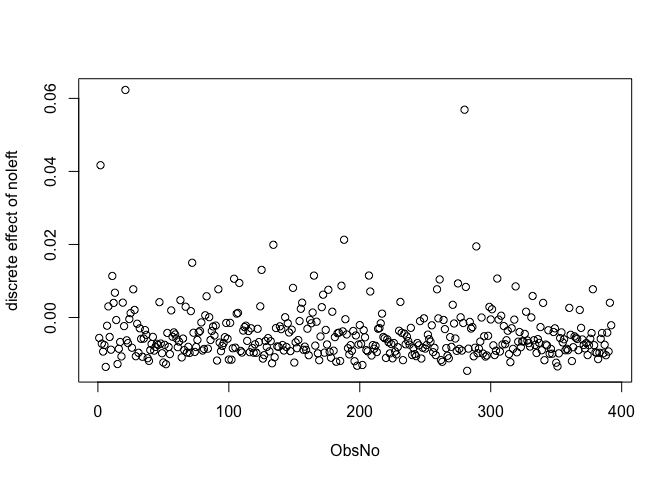
#> [[1]]
#>   [1]   1   2   3   4   5   6   7   8   9  10  11  12  13  14  15  16  17  18
#>  [19]  19  20  21  22  23  24  25  26  27  28  29  30  31  32  33  34  35  36
#>  [37]  37  38  39  40  41  42  43  44  45  46  47  48  49  50  51  52  53  54
#>  [55]  55  56  57  58  59  60  61  62  63  64  65  66  67  68  69  70  71  72
#>  [73]  73  74  75  76  77  78  79  80  81  82  83  84  85  86  87  88  89  90
#>  [91]  91  92  93  94  95  96  97  98  99 100 101 102 103 104 105 106 107 108
#> [109] 109 110 111 112 113 114 115 116 117 118 119 120 121 122 123 124 125 126
#> [127] 127 128 129 130 131 132 133 134 135 136 137 138 139 140 141 142 143 144
#> [145] 145 146 147 148 149 150 151 152 153 154 155 156 157 158 159 160 161 162
#> [163] 163 164 165 166 167 168 169 170 171 172 173 174 175 176 177 178 179 180
#> [181] 181 182 183 184 185 186 187 188 189 190 191 192 193 194 195 196 197 198
#> [199] 199 200 201 202 203 204 205 206 207 208 209 210 211 212 213 214 215 216
#> [217] 217 218 219 220 221 222 223 224 225 226 227 228 229 230 231 232 233 234
#> [235] 235 236 237 238 239 240 241 242 243 244 245 246 247 248 249 250 251 252
#> [253] 253 254 255 256 257 258 259 260 261 262 263 264 265 266 267 268 269 270
#> [271] 271 272 273 274 275 276 277 278 279 280 281 282 283 284 285 286 287 288
#> [289] 289 290 291 292 293 294 295 296 297 298 299 300 301 302 303 304 305 306
#> [307] 307 308 309 310 311 312 313 314 315 316 317 318 319 320 321 322 323 324
#> [325] 325 326 327 328 329 330 331 332 333 334 335 336 337 338 339 340 341 342
#> [343] 343 344 345 346 347 348 349 350 351 352 353 354 355 356 357 358 359 360
#> [361] 361 362 363 364 365 366 367 368 369 370 371 372 373 374 375 376 377 378
#> [379] 379 380 381 382 383 384 385 386 387 388 389 390 391 392
#>
#> [[2]]
#>               noleft
#>   [1,] -5.598288e-03
#>   [2,]  1.947725e-02
#>   [3,] -7.609622e-03
#>   [4,] -9.406895e-03
#>   [5,] -8.263163e-03
#>   [6,] -1.353989e-02
#>   [7,] -2.896787e-03
#>   [8,]  2.406090e-03
#>   [9,] -5.684322e-03
#>  [10,] -8.971304e-03
#>  [11,]  7.715432e-03
#>  [12,]  6.920482e-04
#>  [13,] -1.255324e-03
#>  [14,] -2.233904e-03
#>  [15,] -1.279926e-02
#>  [16,] -8.633075e-03
#>  [17,] -6.763630e-03
#>  [18,] -1.064960e-02
#>  [19,] -1.114169e-04
#>  [20,] -4.248346e-03
#>  [21,]  1.104608e-02
#>  [22,] -6.223970e-03
#>  [23,] -7.119241e-03
#>  [24,] -6.586157e-03
#>  [25,]  9.042696e-04
#>  [26,] -8.323887e-03
#>  [27,]  4.787540e-04
#>  [28,] -5.370501e-04
#>  [29,] -1.073133e-02
#>  [30,] -2.530176e-03
#>  [31,] -1.031445e-02
#>  [32,] -3.039879e-03
#>  [33,] -6.046437e-03
#>  [34,] -1.076181e-02
#>  [35,] -5.909119e-03
#>  [36,] -3.586405e-03
#>  [37,] -4.700915e-03
#>  [38,] -1.117915e-02
#>  [39,] -1.207136e-02
#>  [40,] -9.109931e-03
#>  [41,] -7.396241e-03
#>  [42,] -5.605386e-03
#>  [43,] -9.538402e-03
#>  [44,] -8.209286e-03
#>  [45,] -7.919540e-03
#>  [46,] -7.817731e-03
#>  [47,]  2.999971e-03
#>  [48,] -7.292365e-03
#>  [49,] -9.987204e-03
#>  [50,] -1.235685e-02
#>  [51,] -8.165931e-03
#>  [52,] -1.286344e-02
#>  [53,] -4.606757e-03
#>  [54,] -8.308527e-03
#>  [55,] -1.012591e-02
#>  [56,]  1.821880e-03
#>  [57,] -5.846828e-03
#>  [58,] -4.634362e-03
#>  [59,] -5.031211e-03
#>  [60,] -5.963307e-03
#>  [61,] -8.492299e-03
#>  [62,] -7.244595e-03
#>  [63,] -2.256899e-03
#>  [64,] -1.114899e-02
#>  [65,] -6.521359e-03
#>  [66,] -9.270956e-03
#>  [67,]  2.034223e-03
#>  [68,] -9.783301e-03
#>  [69,] -8.482276e-03
#>  [70,] -1.002258e-02
#>  [71,]  1.230819e-03
#>  [72,]  1.308609e-02
#>  [73,] -5.343419e-03
#>  [74,] -9.636049e-03
#>  [75,] -8.131076e-03
#>  [76,] -6.744983e-03
#>  [77,] -4.713461e-03
#>  [78,] -4.022454e-03
#>  [79,] -1.482202e-03
#>  [80,] -9.478778e-03
#>  [81,] -9.076705e-03
#>  [82,] -4.491019e-04
#>  [83,]  3.684216e-03
#>  [84,] -8.966944e-03
#>  [85,] -9.074431e-04
#>  [86,] -6.162682e-03
#>  [87,] -3.833580e-03
#>  [88,] -4.063911e-03
#>  [89,] -5.316804e-03
#>  [90,] -2.810948e-03
#>  [91,] -1.183545e-02
#>  [92,]  2.310580e-03
#>  [93,] -6.933042e-03
#>  [94,] -9.391608e-03
#>  [95,] -8.042177e-03
#>  [96,] -7.180535e-03
#>  [97,] -6.089510e-03
#>  [98,] -1.851852e-03
#>  [99,] -8.444208e-03
#> [100,] -1.153564e-02
#> [101,] -1.822820e-03
#> [102,] -1.186540e-02
#> [103,] -8.495010e-03
#> [104,]  2.926796e-03
#> [105,] -8.495066e-03
#> [106,] -2.800092e-03
#> [107,]  9.199830e-04
#> [108,]  1.117961e-03
#> [109,] -9.679126e-03
#> [110,] -9.992237e-03
#> [111,] -4.730041e-03
#> [112,] -2.703955e-03
#> [113,] -2.524634e-03
#> [114,] -6.451010e-03
#> [115,] -4.130997e-03
#> [116,] -1.037997e-02
#> [117,] -3.555406e-03
#> [118,] -8.771392e-03
#> [119,] -9.890194e-03
#> [120,] -7.719499e-03
#> [121,] -9.792913e-03
#> [122,] -4.307340e-03
#> [123,] -7.378957e-03
#> [124,]  1.568075e-03
#> [125,]  1.056418e-02
#> [126,] -1.129786e-02
#> [127,] -1.028748e-02
#> [128,] -6.530840e-03
#> [129,] -8.252538e-03
#> [130,] -5.778306e-03
#> [131,] -9.383868e-03
#> [132,] -6.966914e-03
#> [133,] -1.262002e-02
#> [134,]  1.385933e-02
#> [135,] -1.083393e-02
#> [136,] -7.089829e-03
#> [137,] -7.957489e-03
#> [138,] -8.628324e-03
#> [139,] -3.133294e-03
#> [140,] -3.369809e-03
#> [141,] -7.814735e-03
#> [142,] -9.205570e-03
#> [143,] -4.331366e-04
#> [144,] -8.077353e-03
#> [145,] -2.549393e-03
#> [146,] -4.413741e-03
#> [147,] -9.397510e-03
#> [148,] -5.102295e-03
#> [149,]  4.706640e-03
#> [150,] -1.245139e-02
#> [151,] -7.069717e-03
#> [152,] -8.829082e-03
#> [153,] -6.843380e-03
#> [154,] -2.127050e-03
#> [155,]  1.158592e-03
#> [156,]  4.788014e-04
#> [157,] -8.987661e-03
#> [158,] -8.687339e-03
#> [159,] -8.949422e-03
#> [160,] -3.272768e-03
#> [161,] -1.045151e-02
#> [162,] -2.837588e-03
#> [163,] -3.244557e-03
#> [164,]  3.194505e-05
#> [165,]  8.705072e-03
#> [166,] -8.399848e-03
#> [167,] -1.853832e-03
#> [168,] -9.800817e-03
#> [169,] -1.172571e-02
#> [170,] -5.337462e-03
#> [171,]  2.015853e-03
#> [172,]  4.979710e-03
#> [173,] -9.568438e-03
#> [174,] -3.568472e-03
#> [175,] -7.411663e-03
#> [176,]  7.025894e-03
#> [177,] -9.599501e-03
#> [178,] -1.111695e-02
#> [179,]  8.047166e-04
#> [180,] -9.133003e-03
#> [181,] -5.869573e-03
#> [182,] -1.214623e-02
#> [183,] -4.669854e-03
#> [184,] -4.463326e-03
#> [185,] -1.191000e-02
#> [186,]  3.744900e-03
#> [187,] -3.891071e-03
#> [188,]  1.528206e-02
#> [189,] -1.221079e-03
#> [190,] -4.915065e-03
#> [191,] -8.721037e-03
#> [192,] -1.009595e-02
#> [193,] -7.627844e-03
#> [194,] -9.192283e-03
#> [195,] -3.858292e-03
#> [196,] -1.195036e-02
#> [197,] -5.027640e-03
#> [198,] -1.338932e-02
#> [199,] -7.686192e-03
#> [200,] -2.175681e-03
#> [201,] -7.630563e-03
#> [202,] -1.298441e-02
#> [203,] -4.121039e-03
#> [204,] -5.521668e-03
#> [205,] -9.008744e-03
#> [206,] -9.510566e-03
#> [207,]  1.040739e-02
#> [208,]  1.941050e-03
#> [209,] -1.062927e-02
#> [210,] -7.643385e-03
#> [211,] -8.562723e-03
#> [212,] -7.959312e-03
#> [213,] -9.433196e-03
#> [214,] -3.208929e-03
#> [215,] -3.150490e-03
#> [216,] -2.386806e-03
#> [217,] -7.148068e-04
#> [218,] -5.670331e-03
#> [219,] -6.322571e-03
#> [220,] -1.111328e-02
#> [221,] -5.924960e-03
#> [222,] -7.399140e-03
#> [223,] -9.955440e-03
#> [224,] -7.299339e-03
#> [225,] -1.132752e-02
#> [226,] -7.113288e-03
#> [227,] -9.448383e-03
#> [228,] -1.019827e-02
#> [229,] -8.151542e-03
#> [230,] -3.652505e-03
#> [231,]  2.728468e-03
#> [232,] -4.551079e-03
#> [233,] -1.172551e-02
#> [234,] -4.561673e-03
#> [235,] -8.218363e-03
#> [236,] -5.249490e-03
#> [237,] -6.992996e-03
#> [238,] -7.473846e-03
#> [239,] -3.873894e-03
#> [240,] -1.083368e-02
#> [241,] -8.429710e-03
#> [242,] -1.028596e-02
#> [243,] -1.086683e-02
#> [244,] -7.084731e-03
#> [245,] -7.575687e-03
#> [246,] -1.892026e-03
#> [247,] -1.161981e-02
#> [248,] -8.590581e-03
#> [249,] -9.914037e-04
#> [250,] -8.738099e-03
#> [251,] -7.578947e-03
#> [252,] -5.653197e-03
#> [253,] -6.006835e-03
#> [254,] -6.722851e-03
#> [255,] -2.589090e-03
#> [256,] -9.610443e-03
#> [257,] -8.338985e-03
#> [258,] -1.034657e-02
#> [259,]  6.450144e-03
#> [260,] -5.449153e-04
#> [261,]  7.807687e-03
#> [262,] -1.190907e-02
#> [263,] -1.225764e-02
#> [264,] -7.021863e-04
#> [265,] -3.533558e-03
#> [266,] -9.038486e-03
#> [267,] -1.041851e-02
#> [268,] -1.124650e-02
#> [269,] -6.150331e-03
#> [270,] -8.218751e-03
#> [271,]  2.274098e-03
#> [272,] -1.730688e-03
#> [273,] -5.824437e-03
#> [274,] -9.284250e-03
#> [275,]  8.094698e-03
#> [276,] -8.595038e-03
#> [277,] -1.528430e-03
#> [278,] -9.065789e-03
#> [279,] -3.611924e-03
#> [280,]  1.061615e-02
#> [281,]  8.192461e-03
#> [282,] -1.455246e-02
#> [283,] -8.811758e-03
#> [284,] -1.468948e-03
#> [285,] -3.639214e-03
#> [286,] -2.806603e-03
#> [287,] -1.057451e-02
#> [288,] -8.282634e-03
#> [289,]  1.545178e-02
#> [290,] -9.694678e-03
#> [291,] -8.973789e-03
#> [292,] -6.693721e-03
#> [293,] -1.168347e-04
#> [294,] -9.898500e-03
#> [295,] -5.180498e-03
#> [296,] -1.103828e-02
#> [297,] -1.056742e-02
#> [298,] -5.545494e-03
#> [299,]  2.494130e-03
#> [300,] -2.497228e-03
#> [301,]  1.162661e-03
#> [302,] -8.480235e-03
#> [303,] -1.051961e-02
#> [304,] -9.325412e-03
#> [305,]  8.126713e-03
#> [306,] -1.696441e-03
#> [307,] -9.492427e-03
#> [308,]  1.869034e-04
#> [309,] -7.721901e-03
#> [310,] -2.711671e-03
#> [311,] -7.344956e-03
#> [312,] -6.244634e-03
#> [313,] -3.628332e-03
#> [314,] -1.004535e-02
#> [315,] -1.228562e-02
#> [316,] -3.470856e-03
#> [317,] -8.496254e-03
#> [318,] -1.634409e-03
#> [319,]  8.514505e-04
#> [320,] -9.725001e-03
#> [321,] -7.165384e-03
#> [322,] -4.549788e-03
#> [323,] -8.195993e-03
#> [324,] -7.554994e-03
#> [325,] -6.570968e-03
#> [326,] -4.989783e-03
#> [327,]  1.358466e-03
#> [328,] -6.224975e-03
#> [329,] -7.268272e-03
#> [330,] -8.532516e-03
#> [331,] -1.207524e-03
#> [332,]  4.608483e-03
#> [333,] -6.599699e-03
#> [334,] -8.154693e-03
#> [335,] -9.722565e-03
#> [336,] -6.907471e-03
#> [337,] -7.237225e-03
#> [338,] -3.097704e-03
#> [339,] -8.912496e-03
#> [340,]  2.397602e-03
#> [341,] -1.171796e-02
#> [342,] -7.445747e-03
#> [343,] -7.712146e-03
#> [344,] -3.783187e-03
#> [345,] -1.021067e-02
#> [346,] -8.918724e-03
#> [347,] -1.007232e-02
#> [348,] -5.307932e-03
#> [349,] -4.117353e-03
#> [350,] -1.233684e-02
#> [351,] -1.360916e-02
#> [352,] -9.970121e-03
#> [353,] -6.904391e-03
#> [354,] -4.346718e-03
#> [355,] -7.312581e-03
#> [356,] -5.978408e-03
#> [357,] -9.183093e-03
#> [358,] -8.775679e-03
#> [359,] -9.289556e-03
#> [360,]  2.382126e-03
#> [361,] -5.364328e-03
#> [362,] -1.219644e-02
#> [363,] -8.366649e-03
#> [364,] -5.193816e-03
#> [365,] -5.672822e-03
#> [366,] -6.472312e-03
#> [367,] -9.274423e-03
#> [368,]  1.658076e-03
#> [369,] -3.022759e-03
#> [370,] -6.505199e-03
#> [371,] -7.801323e-03
#> [372,] -8.524404e-03
#> [373,] -7.157457e-03
#> [374,] -1.035145e-02
#> [375,] -7.747079e-03
#> [376,] -5.978645e-03
#> [377,] -4.369100e-03
#> [378,]  2.092952e-03
#> [379,] -7.929802e-03
#> [380,] -9.831830e-03
#> [381,] -9.789087e-03
#> [382,] -1.135309e-02
#> [383,] -9.972806e-03
#> [384,] -7.303484e-03
#> [385,] -4.796398e-03
#> [386,] -9.854517e-03
#> [387,] -7.576823e-03
#> [388,] -1.034892e-02
#> [389,] -4.421289e-03
#> [390,] -9.485456e-03
#> [391,] -2.198701e-03
#> [392,] -2.323559e-03With fracreg, fracreghet,
fracregpd, fracregmlogit, and
fracregridge, you have a complete toolkit for modelling
fractional responses bounded between \([0,1]\), regardless of inflation,
endogeneity, unobserved panel effects, multinomial structure, or
multicollinearity.
This package builds upon, consolidates, and modernises the fractional
regression frameworks originally implemented in the frm,
frmhet, and frmpd R packages developed by
Joaquim J.S. Ramalho. As those original packages have been deprecated
and removed from the active CRAN repository, fracreg serves
as an actively maintained successor, ensuring these econometric tools
remain available to the R community.
Furthermore, we acknowledge James Ji (@f1kidd) and A. John Woodill (@johnwoodill), the
authors of the fmlogit R package on GitHub, whose
foundational work on fractional multinomial logit models inspired the
implementation of fracregmlogit. We also extend our
gratitude to Ariel Rokem and Kendrick Kay, the authors of the
fracridge package, whose methodological contributions to
fractional ridge regression are incorporated into the
fracregridge functionalities of this package.
Ji, J., and Woodill, A. J. fmlogit: Fractional Multinomial Logit. R package repository. https://github.com/f1kidd/fmlogit
Rokem, A., and Kay, K. fracridge: Fractional Ridge Regression. Package repository. https://github.com/nrdg/fracridge
Ramalho, J. J. S. (2022). frm: Fractional Regression Models. R package. Formerly available on CRAN, currently archived.
Ramalho, J. J. S. (2023). frmhet: Fractional Regression Models under Heterogeneity. R package. Formerly available on CRAN, currently archived.
Ramalho, J. J. S. (2023). frmpd: Fractional Regression Models for Panel Data. R package. Formerly available on CRAN, currently archived.
Buis, M. L. (2008). “fmlogit: Stata module fitting a fractional multinomial logit model by quasi maximum likelihood”, Statistical Software Components, Boston College Department of Economics.
Mullahy, J. (2015). “Multivariate fractional regression estimation of econometric share models”, Journal of Econometric Methods, 4(1), 71-100.
Murteira, J. M. R., and Ramalho, J. J. S. (2016). “Regression analysis of multivariate fractional data”, Econometric Reviews, 35(4), 515-552.
Papke, L. E. and Wooldridge, J. M. (1996). “Econometric methods for fractional response variables with an application to 401(k) plan participation rates”, Journal of Applied Econometrics, 11(6), 619-632.
Papke, L. E., & Wooldridge, J. M. (2008). “Panel data methods for fractional response variables with an application to test pass rates”, Journal of Econometrics, 145(1-2), 121-133.
Ramalho, E. A., & Ramalho, J. J. S. (2017). “Moment-based estimation of nonlinear regression models with boundary outcomes and endogeneity, with applications to nonnegative and fractional responses”, Econometric Reviews, 36(4), 397-420.
Ramalho, E.A., Ramalho, J.J.S. and Murteira, J.M.R. (2011). “Alternative estimating and testing empirical strategies for fractional response models”, Journal of Economic Surveys, 25(1), 19-68.
Ramalho, E.A., Ramalho, J.J.S. and Murteira, J.M.R. (2014). “A generalized goodness-of-functional form test for binary and fractional response models”, Manchester School, 82(4), 488-507.
Ramsey, J.B. (1969). “Tests for Specification Errors in Classical Linear Least-Squares Regression Analysis”, Journal of the Royal Statistical Society: Series B (Methodological), 31(2), 350-371.
Rokem, A., & Kay, K. (2020). “Fractional ridge regression: a fast, interpretable reparameterization of ridge regression”, GigaScience, 9(12).
For more information, please visit the package website or file an issue on GitHub.
To cite this package in your research:
citation("fracreg")These binaries (installable software) and packages are in development.
They may not be fully stable and should be used with caution. We make no claims about them.