The hardware and bandwidth for this mirror is donated by METANET, the Webhosting and Full Service-Cloud Provider.
If you wish to report a bug, or if you are interested in having us mirror your free-software or open-source project, please feel free to contact us at mirror[@]metanet.ch.
![]()
![]()
![]()
![]()
This package “gamutil” provides some short-cut functions to facilitate to work with mgcv::gam and mgcv::bam.
You can install the development version of gamutil from GitHub:
# install.packages("devtools")
devtools::install_github("msaito8623/gamutil")In the current version, the main function of gamutil is gamutil::plot_contour. The function takes a mgcv::gam object and returns a ggplot object, automating the whole process of making a new data frame, calculating the model’s predictions, and constructing a contour plot using ggplot.
Suppose you fitted the following model, using mgcv::gam:
library(mgcv)
#> Loading required package: nlme
#> This is mgcv 1.9-4. For overview type '?mgcv'.
print(mdl$formula)
#> y ~ s(x0) + s(x1) + s(x2) + ti(x0, x1) + ti(x0, x2) + ti(x1,
#>     x2) + ti(x0, x1, x2)
Then, you can visualize estimated effects of “x1” and “x2” as below:
library(gamutil)
plt <- plot_contour(mdl, view=c('x1','x2'))
print(plt)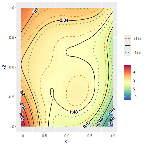
But there are already several functions available for similar purposes. For example, there are mgcv::vis.gam and itsadug::fvisgam for visualizing summed effects. For partial effects, mgcv::plot.gam and itsadug::pvisgam can be used. There are intermediate cases between summed effects and partial effects, which I would call “partially-summed effects”. Partially summed effects refer to the sum of the effects by only several partial effects.
For example, suppose we are interested in the effects of “x1” and “x2”. There are several terms containing “x1” and “x2” in the current model (fitted above). If we visualize summed effects, all the terms would be included, including those without “x1” or “x2”, for example “s(x)”. In contrast, if we choose to visualize partial effects, we have to choose one of the terms that contain “x1” and/or “x2”. How can we specify the sum of the partial effects of “s(x1)”, “s(x2)”, and “ti(x1,x2)”? It can be achieved by gamutil::plot_contour:
plt <- plot_contour(mdl, view=c('x1','x2'), summed=FALSE, terms.size='medium', verbose=TRUE)
#> Selected:
#> s(x1)
#> s(x2)
#> ti(x1,x2)
print(plt)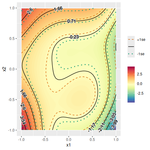
With “terms.size=‘medium’”, all the terms that contain the variables specified in “view” but not any other variable would be included. But, how about “ti(x0,x1)”, “ti(x0,x2)”, and “ti(x0,x1,x2)”? They do contain uninterested variables (i.e., “x0”). But, they also include the variables of interest. To include all the terms that contain at least one variable of interest specified in “view”, you only need to set “terms.size=‘max’”:
plt <- plot_contour(mdl, view=c('x1','x2'), summed=FALSE, terms.size='max', verbose=TRUE)
#> Selected:
#> s(x1)
#> s(x2)
#> ti(x0,x1)
#> ti(x0,x2)
#> ti(x1,x2)
#> ti(x0,x1,x2)
print(plt)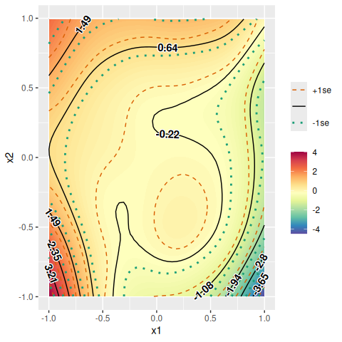
The other possible value for “terms.size” is “min”, which would plot a partial-effect plot:
plt <- plot_contour(mdl, view=c('x1','x2'), summed=FALSE, terms.size='min', verbose=TRUE)
#> Selected:
#> ti(x1,x2)
print(plt)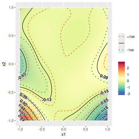
If you need a summed-effect plot, you can set “summed=TRUE”:
plt <- plot_contour(mdl, view=c('x1','x2'), summed=TRUE, verbose=TRUE)
#> Selected: All (summed effect).
print(plt)
The argument “axis.len” controls resolution of the contour plot to be produced (default=50). Bigger numbers for the argument would draw smoother contour lines.
plt <- plot_contour(mdl, view=c('x1','x2'), axis.len=10)
print(plt)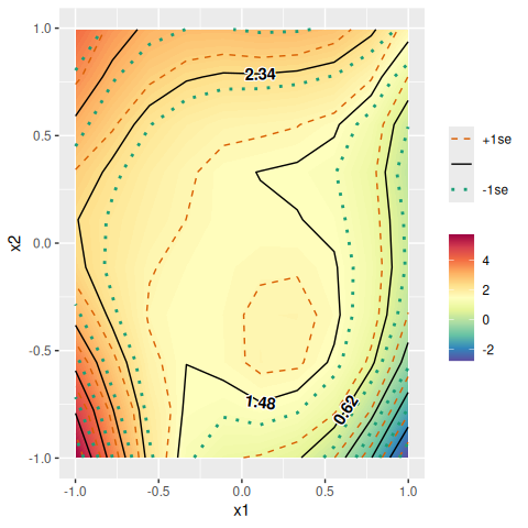
The interval between contour lines can be adjusted by the “break.interval” argument.
plt <- plot_contour(mdl, view=c('x1','x2'), axis.len=100, break.interval=1.5)
print(plt)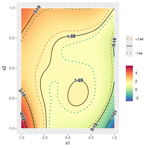
The return value of gamutil::plot_contour is a ggplot object. Therefore, it can be modified in the same way as you would do for ggplot objects in general. For example, you can change font sizes and a plot title as below:
library(ggplot2)
plt <- plot_contour(mdl, view=c('x1','x2'), verbose=TRUE)
#> Selected: All (summed effect).
plt <- plt + theme(text=element_text(size=25))
plt <- plt + labs(title='Summed effects')
plt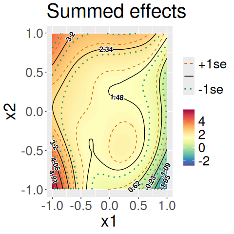
If you have a by-variable in some terms in a model, you can produce contour plots separately for each level of the by-variable.
print(mdl_fac$formula)
#> y ~ s(x1, by = fac) + s(x2, by = fac) + ti(x1, x2, by = fac)
plt <- plot_contour(mdl_fac, view=c('x1','x2'), cond=list(fac=c("A","B")))
print(plt)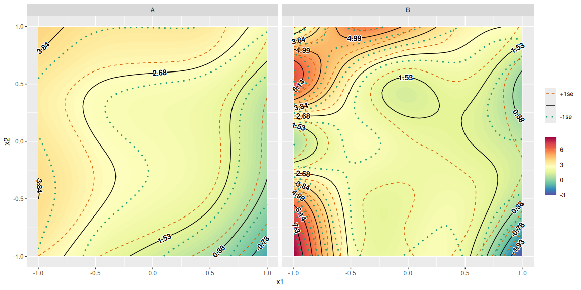
Make sure to always specify the level(s) of the by-variable if you have a by-variable in a model. This is because mgcv::gam would estimate separate smooths/surfaces for each level of a by-variable. In other words, there is no intermediate or average smooth or surface in such a case. As a consequence, if you don’t specify any level of a by-variable, gamutil::plot_contour cannot know which level to plot and therefore produces an error:
plt <- plot_contour(mdl, view=c('x1','x2'), cond=list())Some functions in this package, especially gamutil::plot_contour, are inspired by mgcv::vis.gam, mgcv::plot.gam, itsadug::fvisgam, and itsadug::pvisgam.
These binaries (installable software) and packages are in development.
They may not be fully stable and should be used with caution. We make no claims about them.