The hardware and bandwidth for this mirror is donated by METANET, the Webhosting and Full Service-Cloud Provider.
If you wish to report a bug, or if you are interested in having us mirror your free-software or open-source project, please feel free to contact us at mirror[@]metanet.ch.
![]()
![]()
ggincerta is an extension of ggplot2 that introduces new layers and scales for visualizing spatial uncertainty, and can be extended to more general bivariate schemes. It reimplements the visualisation methods for three types of maps introduced in the Vizumap package in a way that fully aligns with the grammar of graphics and integrates seamlessly with the ggplot2 ecosystem. It makes the visualisation process more flexible and convenient, while also adding additional visualisation options.
# Install the release from CRAN:
install.packages("ggincerta")

# Install the development version from GitHub:
# install.packages("pak")
pak::pak("maggiexma/ggincerta")The example dataset included in ggincerta is an sf object adapted
from the nc shapefile in the sf package. It contains two
simulated columns value and sd, which are mainly used in example maps to
demonstrate how to visualise regional uncertainty alongside average
estimates. For more details about the description and design of three
map types, see https://doi.org/10.1002/sta4.150.
library(ggincerta)
#> Loading required package: ggplot2
The ggincerta package defines a new scale function,
scale_*_bivariate(), for creating bivariate colour mapping
schemes that work with geom_sf(). In the data space, two
variables are discretised into n_breaks bins, forming
crossed combinations that are mapped to a colour grid. Each cell in the
colour grid is generated through a chosen mixture of visual properties,
such as hue, lightness, saturation, or opacity.
ggplot(nc) + geom_sf(aes(fill = duo(value, sd)))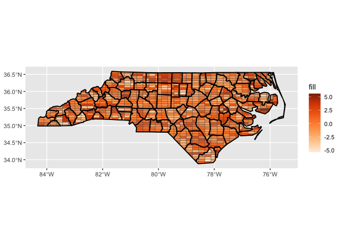
The figure above shows the default visual effect of
scale_*_bivariate(), where colours are generated by
additive mixing in RGB space between two hue-based lightness gradient
ramps. Another option is to use the provided
bivar_fade_palette() to specify colours for the value
dimension, while progressively suppressing another perceptual dimension
along the uncertainty axis.
ggplot(nc) + geom_sf(aes(fill = duo(value, sd))) +
  scale_fill_bivariate(palette_fun = bivar_fade_palette,
                       colours = c("#F6E8C3", "orange", "red"),
                       palette_params = list(fade = "desaturate"))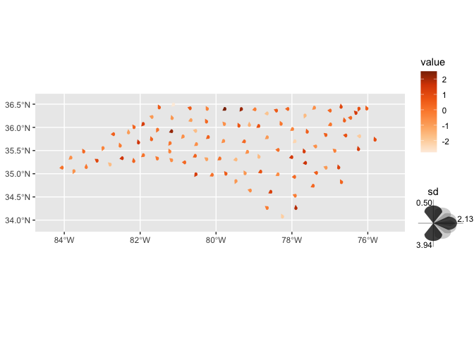
Value-Suppressing Uncertainty Palettes proposed by Correll et
al. (2018) can be implemented by scale_*_vsup() in
ggincerta. The main idea is to suppress colour variation in regions with
higher uncertainty, thereby directing visual attention towards more
reliable value differences.
ggplot(nc) +
  geom_sf(aes(fill = duo(value, sd))) +
  scale_fill_vsup(
    breaks = list(
      seq(-3, 3, length.out = 9),
      seq(0, 4, length.out = 5)
    ),
    limits = list(
      c(-3, 3),
      c(0, 4)
    )
  ) + theme(legend.text = element_text(size = 7))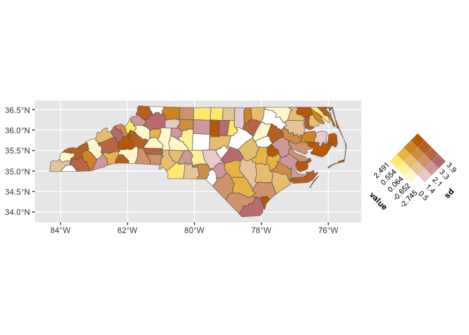
ggincerta defines two layer functions geom_sf_pixel()
and geom_sf_glyph() for creating pixel and glyph maps,
respectively. They can be used in the same way as other
geom_*() functions in ggplot2, like
geom_point().
ggplot(nc) + geom_sf_pixel(mapping = aes(fill = duo_pixel(value, sd)), seed = 123)
#> geom_sf_pixel_new(): input data has a geographic CRS and sf is using s2; pixelation may be slow. Consider transforming to a projected planar CRS first.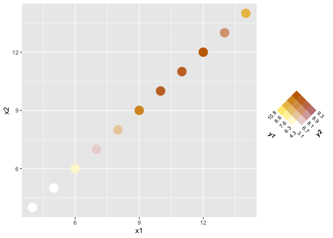
Each unit region in a pixel map is tessellated into pixels. Pixel
values are sampled from a specified probability distribution
parameterised by v1 and v2 for each region,
and are then mapped to the colour aesthetic. Greater variation in pixel
colours within a region indicates higher uncertainty.
Glyph maps are essentially centroid maps. ggincerta provides glyphs
with different shapes and corresponding aesthetics for simultaneously
visualising value and uncertainty. One option uses regular shapes,
including circles, squares, triangles, and hexagons, which can work
together with scale_colour_bivariate().
ggplot(nc) + geom_sf_glyph(mapping = aes(colour = duo(value, sd)))
#> Warning: st_point_on_surface assumes attributes are constant over geometries
#> Warning in st_point_on_surface.sfc(st_geometry(x)): st_point_on_surface may not
#> give correct results for longitude/latitude data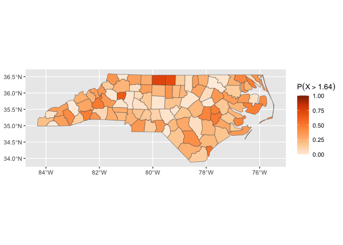
Another type of glyph is drop-shaped, where uncertainty is
represented by the rotation angle through the newly introduced
angle aesthetic.
ggplot(nc) +
  geom_sf_glyph(aes(colour = value, angle = sd), shape = "drop")
#> Warning: st_point_on_surface assumes attributes are constant over geometries
#> Warning in st_point_on_surface.sfc(st_geometry(x)): st_point_on_surface may not
#> give correct results for longitude/latitude data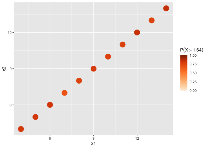
The remaining glyph form is the Chernoff face, originally proposed by Herman Chernoff (1973), which uses human facial expressions to represent multivariate values. The implementation in ggincerta builds upon the grob and scale design provided by the ggChernoff package. In the example below, facial colour is mapped to the estimated value, while facial expression conveys uncertainty in an intuitive and perceptually meaningful manner: lower uncertainty produces smiling faces, whereas higher uncertainty results in frowning faces.
ggplot(nc) +
  geom_sf_glyph(aes(colour = value, smile = sd), shape = "chernoff")
#> Warning in st_point_on_surface.sfc(data$geometry): st_point_on_surface may not
#> give correct results for longitude/latitude data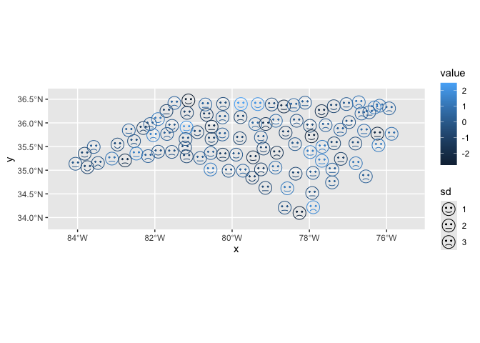
The final visualisation type in ggincerta is the dual map, which
combines a glyph map with a conventional colour-filled choropleth map in
a two-layer display. This design allows two variables to be represented
using separate mappings, scales, and guides, so that their original
values remain directly interpretable. At the same time, it preserves the
ability of the choropleth layer to show the spatial trend of the primary
variable. In addition, it supports the duo() mapping and
can therefore be used together with scale_bivariate() to
achieve three-variable visualisation within a single map.
ggplot(nc) + geom_sf_dualmap(aes(fill = sd, colour = value))
#> Warning: st_point_on_surface assumes attributes are constant over geometries
#> Warning in st_point_on_surface.sfc(st_geometry(x)): st_point_on_surface may not
#> give correct results for longitude/latitude data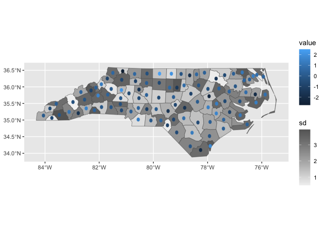
These binaries (installable software) and packages are in development.
They may not be fully stable and should be used with caution. We make no claims about them.