The hardware and bandwidth for this mirror is donated by METANET, the Webhosting and Full Service-Cloud Provider.
If you wish to report a bug, or if you are interested in having us mirror your free-software or open-source project, please feel free to contact us at mirror[@]metanet.ch.

hcinfer

hcinfer provides heteroskedasticity-consistent covariance estimators and normal Wald inference for ordinary least squares models, together with feasible generalized least squares under multiplicative heteroskedasticity for linear regressions. The currently implemented covariance matrix estimators are listed below.

Implemented estimators

The table below is generated by hc_methods() and lists the covariance matrix estimators currently implemented in hcinfer.

Installation

# Official CRAN installation of the package
install.packages("hcinfer")

# r-universe installation
install.packages('hcinfer', repos = c('https://prdm0.r-universe.dev', 'https://cloud.r-project.org'))

# Development version installation from GitHub
remotes::install_github("prdm0/hcinfer", force = TRUE)

Basic use

library(hcinfer)

schools <- PublicSchools
schools$income_scaled <- schools$income / 10000
schools$income_scaled_sq <- schools$income_scaled^2

fit <- lm(expenditure ~ income_scaled + income_scaled_sq, data = schools)

result <- hcinfer(fit)

The default estimator is HCbeta. Use tests() and confint() to extract the main inferential quantities as tibbles.

HCbeta exposes six tuning controls (c1, c2, lower, upper, a_max, b_max); see vignette("hcinfer-hcbeta", package = "hcinfer").

tests(result)
#> # A tibble: 3 × 8
#>   term             estimate null_value std_error z_value p_value alpha reject
#>   <chr>               <dbl>      <dbl>     <dbl>   <dbl>   <dbl> <dbl> <lgl> 
#> 1 (Intercept)          833.          0      851.   0.979   0.328  0.05 FALSE 
#> 2 income_scaled      -1834.          0     2309.  -0.794   0.427  0.05 FALSE 
#> 3 income_scaled_sq    1587.          0     1547.   1.03    0.305  0.05 FALSE
confint(result)
#> # A tibble: 3 × 4
#>   term             conf_low conf_high level
#>   <chr>               <dbl>     <dbl> <dbl>
#> 1 (Intercept)         -834.     2500.  0.95
#> 2 income_scaled      -6359.     2691.  0.95
#> 3 income_scaled_sq   -1446.     4620.  0.95

Confidence intervals

The plot() method displays the robust confidence intervals and marks the null value used in the tests.

plot(result)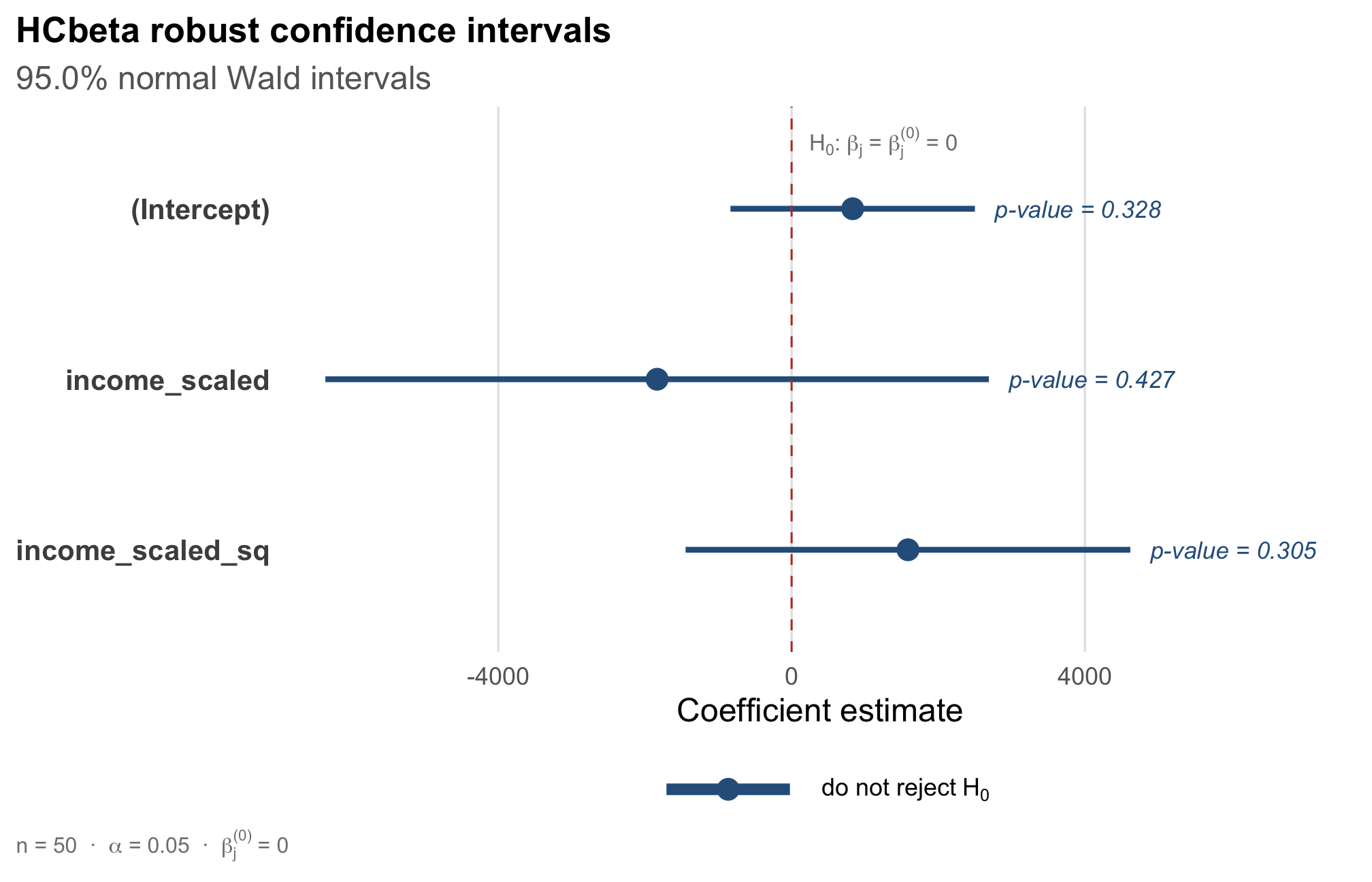

Diagnostics

Use vcov_hc() when you only need the robust covariance matrix and its diagnostics. The plot() method for this object shows leverage values and HC adjustment factors.

cov_hcbeta <- vcov_hc(fit)
plot(cov_hcbeta)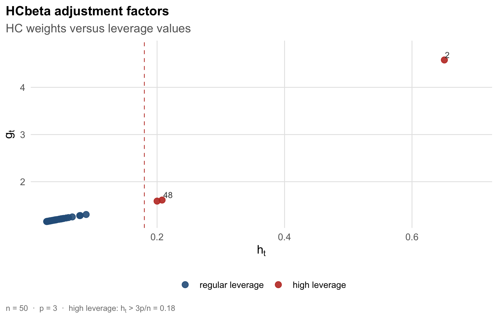

Feasible GLS under multiplicative heteroskedasticity

gls_mult() fits a linear model by feasible generalized least squares when the conditional variance is modelled as an exponential function of dispersion regressors. Maximum likelihood is the default, and Harvey’s two-step estimator is also available.

fit <- lm(expenditure ~ income, data = PublicSchools)

# Maximum likelihood FGLS (default); AIC()/BIC() work via logLik()
gls_fit <- gls_mult(fit)
coef(gls_fit)                       # mean coefficients
coef(gls_fit, model = "dispersion") # log-variance coefficients
AIC(gls_fit); BIC(gls_fit)

# Harvey two-step estimator
gls_mult(fit, estimator = "two_step")

Maximum likelihood fits support logLik(), AIC(), and BIC() (with df = p + q), whereas the two-step fit does not, because its likelihood is not maximized.

Learn more

The package documentation is organized as a progressive learning path. vignette("introduction", package = "hcinfer") covers the API and a typical workflow. vignette("hcinfer-hcbeta", package = "hcinfer") dives into the HCbeta estimator: its parameters, diagnostics, and sensitivity controls. vignette("hcinfer-methodology", package = "hcinfer") presents the statistical methodology behind all HC estimators and the HCbeta motivation. vignette("hcinfer-comparison", package = "hcinfer") compares HCbeta with classical HC estimators on real data. vignette("hcinfer-bootstrap", package = "hcinfer") describes the bootstrap companion for resampling-based inference. Finally, vignette("hcinfer-gls", package = "hcinfer") explains feasible generalized least squares under multiplicative heteroskedasticity.

References

• White, H. (1980). A heteroskedasticity-consistent covariance matrix estimator and a direct test for heteroskedasticity. Econometrica, 48(4), 817-838. doi:10.2307/1912934.
• Cribari-Neto, F. (2004). Asymptotic inference under heteroskedasticity of unknown form. Computational Statistics and Data Analysis, 45(2), 215-233. doi:10.1016/S0167-9473(02)00366-3.
• Cribari-Neto, F. and da Silva, W. B. (2011). A new heteroskedasticity-consistent covariance matrix estimator for the linear regression model. AStA Advances in Statistical Analysis, 95(2), 129-146. doi:10.1007/s10182-010-0141-2.
• Cunha, M. A., Cribari-Neto, F., and Marinho, P. R. D. (manuscript). A beta-based heteroskedasticity-consistent covariance matrix estimator.

See vignette("hcinfer-methodology", package = "hcinfer") for the complete reference list.

These binaries (installable software) and packages are in development.
They may not be fully stable and should be used with caution. We make no claims about them.