The hardware and bandwidth for this mirror is donated by METANET, the Webhosting and Full Service-Cloud Provider.
If you wish to report a bug, or if you are interested in having us mirror your free-software or open-source project, please feel free to contact us at mirror[@]metanet.ch.
An R package for processing data and automatically assessing heartbeat frequency, specifically designed for use with ElectricBlue’s PULSE systems (https://electricblue.eu/pulse).
You can install the development version of heartbeatr from GitHub with:
# install.packages("devtools")
devtools::install_github("coastalwarming/heartbeatr")library(heartbeatr)# here we use the package's example data
paths <- pulse_example()
basename(paths)
#> [1] "20241001_105133.CSV" "20241001_110000.CSV"# to use your own data just get the paths to your target files
paths <- dir("folder_with_your_files")
# but make sure they correspond to a single experiment/device !!
# if in doubt, check the helpfile for the PULSE() function
# [section: One experiment] to better understand what this means
?PULSE Use the step-by-step approach to better understand, debug or fine-tune your workflow
pulse_data <- pulse_read(
  paths,
  msg = FALSE
  )

pulse_data_split <- pulse_split(
   pulse_data,
   window_width_secs = 30,
   window_shift_secs = 60,
   min_data_points = 0.8,
   msg = FALSE
   )

pulse_data_optimized <- pulse_optimize(
  pulse_data_split,
  interpolation_freq = 40,
  bandwidth = 0.75,
  raw_v_smoothed = FALSE,
  multi = TRUE
  )

heart_rates <- pulse_heart(
  pulse_data_optimized
  )

heart_rates <- pulse_doublecheck(
  heart_rates
  )

heart_rates <- pulse_choose_keep(
  heart_rates
)The wrapper function is much simpler to use and delivers exactly the same results (it is just executing the step-by-step workflow at once).
heart_rates2 <- PULSE(
  paths,
  window_width_secs  = 30,
  window_shift_secs  = 60,
  min_data_points    = 0.8,
  interpolation_freq = 40,
  bandwidth          = 0.75,
  raw_v_smoothed     = FALSE
  )

identical(heart_rates, heart_rates2)
#> [1] TRUE
Once processed, PULSE data is stored as a tibble with an average heart rate frequency for each channel/split window. The time is relative to the mid-point of the window. Frequencies are expressed in Hz (multiply by 60 to get BPM). In addition, the following information is also provided, which can be used to classify or filter the data: n, the number of identified heart beats, sd, the standard deviation of the intervals between each pair of consecutive peaks, and ci, the confidence interval of the Hz estimate (hz ± ci).
heart_rates
#> # A tibble: 130 × 12
#>        i smoothed id    time                    data        hz     n    sd    ci
#>    <int> <lgl>    <chr> <dttm>                  <list>   <dbl> <int> <dbl> <dbl>
#>  1     1 TRUE     c01   2024-10-01 10:52:14.985 <tibble> 0.183     5 1.88  3.68
#>  2     1 TRUE     c02   2024-10-01 10:52:14.985 <tibble> 0.18      5 2.88  5.64
#>  3     1 TRUE     c03   2024-10-01 10:52:14.985 <tibble> 0.313     9 0.587 1.15
#>  4     1 TRUE     c04   2024-10-01 10:52:14.985 <tibble> 0.389    11 0.307 0.601
#>  5     1 TRUE     c05   2024-10-01 10:52:14.985 <tibble> 0.36      9 0.86  1.69
#>  6     1 TRUE     c06   2024-10-01 10:52:14.985 <tibble> 0.405    12 0.042 0.083
#>  7     1 TRUE     c07   2024-10-01 10:52:14.985 <tibble> 0.283     8 1.71  3.35
#>  8     1 TRUE     c08   2024-10-01 10:52:14.985 <tibble> 0.115     4 0.114 0.224
#>  9     1 TRUE     c09   2024-10-01 10:52:14.985 <tibble> 0.293     8 0.888 1.74
#> 10     1 TRUE     c10   2024-10-01 10:52:14.985 <tibble> 0.165     5 1.02  2.00
#> # ℹ 120 more rows
#> # ℹ 3 more variables: d_r <dbl>, d_f <lgl>, keep <lgl>
The original data corresponding to each split window is still available.
hr <- heart_rates$data[[1]]
hr
#> # A tibble: 1,200 × 3
#>    time                      val peak
#>    <dttm>                  <dbl> <lgl>
#>  1 2024-10-01 10:52:00.007 2512. FALSE
#>  2 2024-10-01 10:52:00.032 2500. FALSE
#>  3 2024-10-01 10:52:00.057 2486. FALSE
#>  4 2024-10-01 10:52:00.082 2472. FALSE
#>  5 2024-10-01 10:52:00.107 2457. FALSE
#>  6 2024-10-01 10:52:00.132 2441. FALSE
#>  7 2024-10-01 10:52:00.157 2424. FALSE
#>  8 2024-10-01 10:52:00.182 2407. FALSE
#>  9 2024-10-01 10:52:00.207 2389. FALSE
#> 10 2024-10-01 10:52:00.232 2370. FALSE
#> # ℹ 1,190 more rowsThe timestamps corresponding to the peaks identified in each split window can easily be extracted.
head(hr$time[hr$peak])
#> [1] "2024-10-01 10:52:03.830 UTC" "2024-10-01 10:52:08.952 UTC"
#> [3] "2024-10-01 10:52:15.472 UTC" "2024-10-01 10:52:19.295 UTC"
#> [5] "2024-10-01 10:52:27.489 UTC"
Notice that the timestamps are set for UTC +0. This is because the PULSE system ALWAYS records data in UTC +0 because it is much safer from a programming standpoint (no daylight saving time, no leap seconds, etc) and from a user experience standpoint (no mistakes or confusion about which time zone was used when data was collected).
Crucially, you can always convert to the relevant time zone afterwards.
LOCAL_heart_rates <- heart_rates
LOCAL_heart_rates$time <- as.POSIXct(LOCAL_heart_rates$time, tz = Sys.timezone())

# UTC +0
head(heart_rates$time)
#> [1] "2024-10-01 10:52:14.985 UTC" "2024-10-01 10:52:14.985 UTC"
#> [3] "2024-10-01 10:52:14.985 UTC" "2024-10-01 10:52:14.985 UTC"
#> [5] "2024-10-01 10:52:14.985 UTC" "2024-10-01 10:52:14.985 UTC"

# local time zone
head(LOCAL_heart_rates$time)
#> [1] "2024-10-01 11:52:14.985 WEST" "2024-10-01 11:52:14.985 WEST"
#> [3] "2024-10-01 11:52:14.985 WEST" "2024-10-01 11:52:14.985 WEST"
#> [5] "2024-10-01 11:52:14.985 WEST" "2024-10-01 11:52:14.985 WEST"keep columnAfter the dataset has been processed, an additional column is present
in the output: the keepcolumn. This is a logical vector
indicating whether or not each time window should be kept for subsequent
analysis. A given window is deemed as keep == FALSE when
the number of peaks identified falls below the value set for
N and the sd of the intervals between consecutive peaks
exceeds the value supplied to SD. It should be regarded as
a first classification of data points based on quality, but the original
values for n and sdare kept so that the user
can reassess the classification if needed.
heart_rates[,-c(2,5)]
#> # A tibble: 130 × 10
#>        i id    time                       hz     n    sd    ci   d_r d_f   keep
#>    <int> <chr> <dttm>                  <dbl> <int> <dbl> <dbl> <dbl> <lgl> <lgl>
#>  1     1 c01   2024-10-01 10:52:14.985 0.183     5 1.88  3.68  0     FALSE FALSE
#>  2     1 c02   2024-10-01 10:52:14.985 0.18      5 2.88  5.64  0     FALSE FALSE
#>  3     1 c03   2024-10-01 10:52:14.985 0.313     9 0.587 1.15  0.5   FALSE TRUE
#>  4     1 c04   2024-10-01 10:52:14.985 0.389    11 0.307 0.601 0.143 FALSE TRUE
#>  5     1 c05   2024-10-01 10:52:14.985 0.36      9 0.86  1.69  0.5   FALSE FALSE
#>  6     1 c06   2024-10-01 10:52:14.985 0.405    12 0.042 0.083 0.75  FALSE TRUE
#>  7     1 c07   2024-10-01 10:52:14.985 0.283     8 1.71  3.35  0     FALSE FALSE
#>  8     1 c08   2024-10-01 10:52:14.985 0.115     4 0.114 0.224 0     FALSE TRUE
#>  9     1 c09   2024-10-01 10:52:14.985 0.293     8 0.888 1.74  0     FALSE FALSE
#> 10     1 c10   2024-10-01 10:52:14.985 0.165     5 1.02  2.00  0     FALSE FALSE
#> # ℹ 120 more rows
It can be used to filter out poor quality data (note that fewer rows remain).
heart_rates[heart_rates$keep,]
#> # A tibble: 54 × 12
#>        i smoothed id    time                    data        hz     n    sd    ci
#>    <int> <lgl>    <chr> <dttm>                  <list>   <dbl> <int> <dbl> <dbl>
#>  1     1 TRUE     c03   2024-10-01 10:52:14.985 <tibble> 0.313     9 0.587 1.15
#>  2     1 TRUE     c04   2024-10-01 10:52:14.985 <tibble> 0.389    11 0.307 0.601
#>  3     1 TRUE     c06   2024-10-01 10:52:14.985 <tibble> 0.405    12 0.042 0.083
#>  4     1 TRUE     c08   2024-10-01 10:52:14.985 <tibble> 0.115     4 0.114 0.224
#>  5     2 TRUE     c04   2024-10-01 10:53:15.014 <tibble> 0.378    11 0.107 0.21
#>  6     2 TRUE     c06   2024-10-01 10:53:15.014 <tibble> 0.423    12 0.091 0.178
#>  7     3 TRUE     c01   2024-10-01 10:54:14.993 <tibble> 0.406    11 0.546 1.07
#>  8     3 TRUE     c03   2024-10-01 10:54:14.993 <tibble> 0.13      4 0.13  0.254
#>  9     3 TRUE     c04   2024-10-01 10:54:14.993 <tibble> 0.385    11 0.166 0.326
#> 10     3 TRUE     c06   2024-10-01 10:54:14.993 <tibble> 0.427    12 0.127 0.249
#> # ℹ 44 more rows
#> # ℹ 3 more variables: d_r <dbl>, d_f <lgl>, keep <lgl>It’s important to check the quality of the data and of the heart beat frequency estimates.
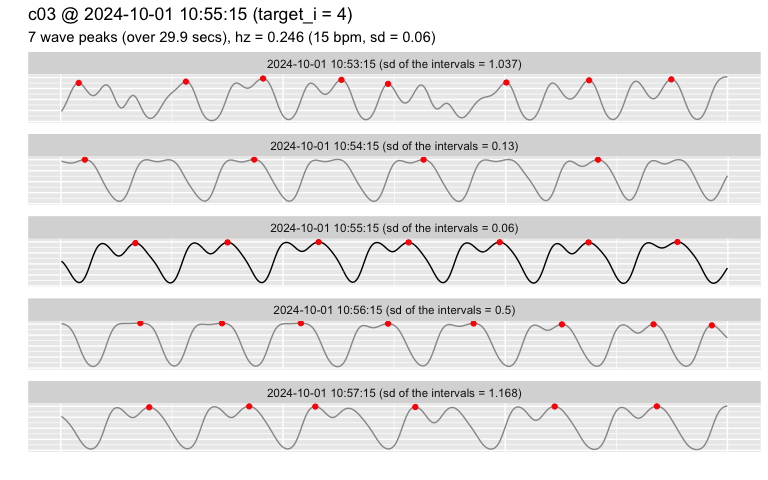
The first step if to inspect the raw data.
# the split window for channel "limpet_1" nearest to target_time is shown in the center:
#   - 2 more windows are shown before/after the target (because range was set to 2)
#   - red dots show where the algorithm detected a peak
pulse_plot_raw(heart_rates,
               ID = "c03",
               target_time = "2024-10-01 10:55",
               range = 2)
Beware of the quality of the original data!
Estimates of heart beat frequency are ALWAYS produced, but they may not be usable at all if the quality of the original data was too poor.
# the channel "c10" contains poor-quality data, where visual inspection
# clearly shows that the heart rate wasn't captured in the signal (lack of
# periodicity and inconsistent intervals between the peaks identified)
pulse_plot_raw(heart_rates,
               ID = "c10",
               target_time = "2024-10-01 11:39",
range = 1) 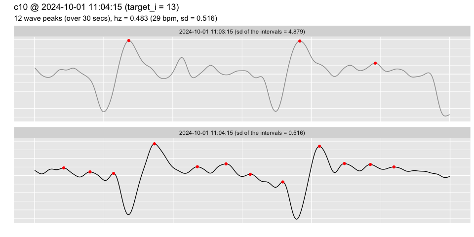
A quick overview of the result of the analysis of the data from all channels:
pulse_plot(heart_rates[heart_rates$id %in% c("c01", "c02", "c03"), ])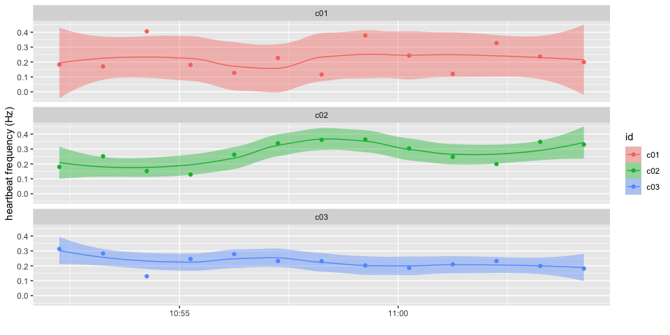
A more detailed view of the channel “c03”, showing the Confidence Interval for each estimate of heart rate.
pulse_plot(heart_rates,
           ID     = "c03",
           smooth = FALSE,
           bpm    = TRUE)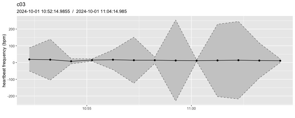
Like humans, invertebrates also show variability in basal heart beat frequencies among individuals. This means that a frequency of 1.5 Hz may be indicative of some stress for an individual whose basal frequency is low (e.g., 0.8), but not so much for another whose basal frequency is already elevated (e.g., 1.2).
To minimize this, heart beat frequencies can be divided by the
average basal frequency, yielding instead a ratio which is independent
of each individual’s basal frequency. Using this ratio
(hz_norm), a value of 0.5 represents a 50% decrease over
basal frequency, and 2.0 represents double the basal frequency - i.e.,
data is now normalized.
In order to properly normalize your dataset, PULSE data should ideally be recorded over a period when all treatments are subjected to the same non-stressful conditions (usually during acclimation). This period is then used to estimate the basal frequency, and all estimates are then divided by that value. The longer and more stable this reference period is, the better, but even 15 minutes may be sufficient in some cases.
# by default, pulse_normalize uses the first 10 mins as the reference period
# here we use 5 mins because the example dataset only spans 50 mins
heart_rates_norm <- pulse_normalize(heart_rates, span = 5)

# a new column is added: hz_norm
head(heart_rates_norm$hz_norm)
#> [1] 0.8575445 0.9240246 1.2520000 1.0547722 1.3196481 0.9588068

# without normalizing
pulse_plot(heart_rates_norm, ID = "c03", normalized = FALSE, facets = FALSE)
# with normalizing
pulse_plot(heart_rates_norm, ID = "c03", normalized = TRUE, facets = FALSE)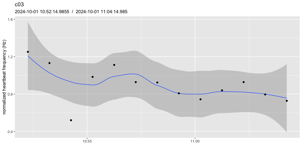
# notice how:
#  - the scale has changed
#  - data points around the initial 5 mins now average to 1.0
#  - the example dataset is not ideal, because the heart beat frequency
#      isn't stable enough over the reference period
pulse_normalize() uses the same period to determine the
basal frequency in all channels. If different channels require different
reference periods, the dataset must be broken into distinct groups and
normalized using their specific set of t0 and
span values. The different groups can then be merged again
using dplyr::bind_rows().
# check the helpfile for the pulse_normalize() function for more details
?pulse_normalizeIt is very common for the quality of the heart beat signal captured with the PULSE system to fluctuate over time. This can be a function of the sensor becoming slightly detached with time, the animal moving its body under the shell, spurious interference from other electronic equipment (especially electronic lighting), and many other factors.
Ultimately, this can be overcome to some extent by collecting data continuously even though a single estimate for each 5 to 15 mins may be sufficient in most experiments (especially the longer ones). In the end, it may be necessary to summarise several heart beat frequency estimates over wider intervals, in effect reducing the number of data points retrieved (and therefore avoiding oversampling).
# before summarising
pulse_plot(heart_rates, ID = "c03")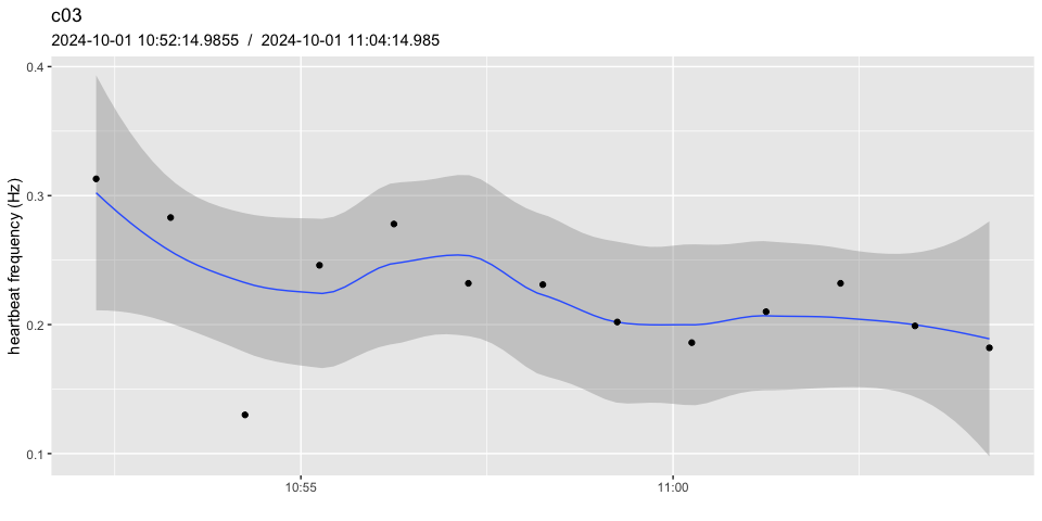
# after summarising
heart_rates_summarised <- pulse_summarise(heart_rates,
                                      FUN = mean,
                                      span_mins = 3,
                                      min_data_points = 0.8)

pulse_plot(heart_rates_summarised, ID = "c03")
#> Warning in simpleLoess(y, x, w, span, degree = degree, parametric = parametric,
#> : span too small.  fewer data values than degrees of freedom.
#> Warning in simpleLoess(y, x, w, span, degree = degree, parametric = parametric,
#> : pseudoinverse used at 1.7278e+09
#> Warning in simpleLoess(y, x, w, span, degree = degree, parametric = parametric,
#> : neighborhood radius 363.6
#> Warning in simpleLoess(y, x, w, span, degree = degree, parametric = parametric,
#> : reciprocal condition number 0
#> Warning in simpleLoess(y, x, w, span, degree = degree, parametric = parametric,
#> : There are other near singularities as well. 1.322e+05
#> Warning in predLoess(object$y, object$x, newx = if (is.null(newdata)) object$x
#> else if (is.data.frame(newdata))
#> as.matrix(model.frame(delete.response(terms(object)), : span too small.  fewer
#> data values than degrees of freedom.
#> Warning in predLoess(object$y, object$x, newx = if (is.null(newdata)) object$x
#> else if (is.data.frame(newdata))
#> as.matrix(model.frame(delete.response(terms(object)), : pseudoinverse used at
#> 1.7278e+09
#> Warning in predLoess(object$y, object$x, newx = if (is.null(newdata)) object$x
#> else if (is.data.frame(newdata))
#> as.matrix(model.frame(delete.response(terms(object)), : neighborhood radius
#> 363.6
#> Warning in predLoess(object$y, object$x, newx = if (is.null(newdata)) object$x
#> else if (is.data.frame(newdata))
#> as.matrix(model.frame(delete.response(terms(object)), : reciprocal condition
#> number 0
#> Warning in predLoess(object$y, object$x, newx = if (is.null(newdata)) object$x
#> else if (is.data.frame(newdata))
#> as.matrix(model.frame(delete.response(terms(object)), : There are other near
#> singularities as well. 1.322e+05
#> Warning in max(ids, na.rm = TRUE): no non-missing arguments to max; returning
#> -Inf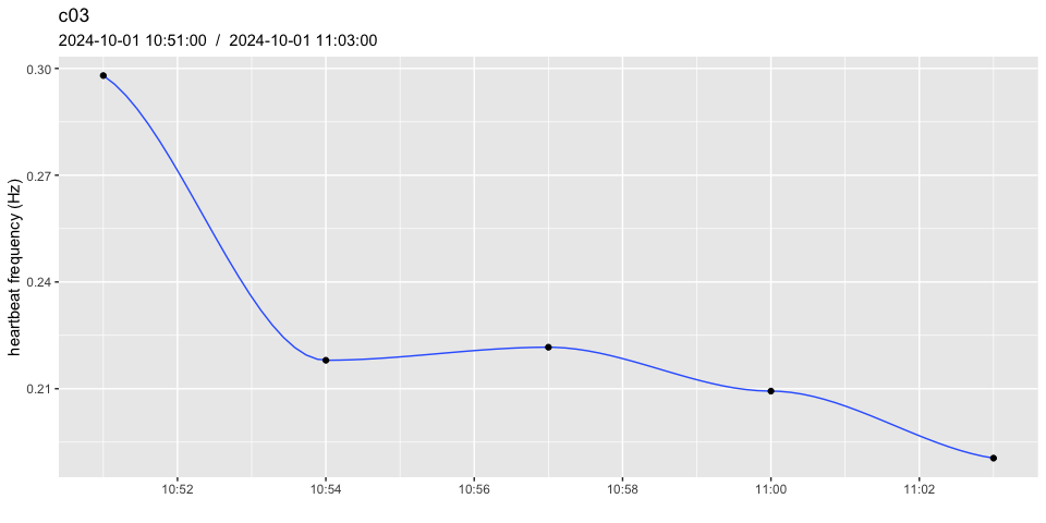
# check the helpfile for the pulse_summarise() function for additional details
?pulse_summarise
These binaries (installable software) and packages are in development.
They may not be fully stable and should be used with caution. We make no claims about them.