The hardware and bandwidth for this mirror is donated by METANET, the Webhosting and Full Service-Cloud Provider.
If you wish to report a bug, or if you are interested in having us mirror your free-software or open-source project, please feel free to contact us at mirror[@]metanet.ch.
The goal of ibdfindr is to detect genomic regions
shared identical by descent (IBD) between two individuals,
using SNP genotypes or genotype likelihoods. It fits continuous-time
hidden Markov models (HMMs) with two- and three-state models for
different relationship types. The main function findIBD()
provides a unified workflow.
ibdfindr was introduced in Vigeland et al. (2026), where it was applied to identify a victim of the 1956 Marcinelle mining disaster in Belgium.
To get the latest official release of ibdfindr, install from CRAN as follows:
install.packages("ibdfindr")For the development version, install from GitHub:
remotes::install_github("magnusdv/ibdfindr")library(ibdfindr)As an example we consider the built-in dataset
cousinsDemo, which contains almost 4000 SNP genotypes for
two related individuals. The data were simulated assuming a relationship
of first cousins. (For details on how the data was generated, the source
code is available in the repository’s folder data-raw.)
head(cousinsDemo)#> CHROM MARKER MB CM A1 A2 FREQ1 ID1 ID2
#> 1 1 rs9442372 1.083324 0.0000000 A G 0.3890 A/G G/G
#> 2 1 rs4648727 1.844830 0.1803812 A C 0.3628 A/C A/C
#> 3 1 rs10910082 2.487496 1.2670505 C T 0.3740 C/T C/T
#> 4 1 rs6695131 3.084360 1.9782286 C T 0.5719 C/T C/T
#> 5 1 rs3765703 3.675872 4.8403127 G T 0.4058 G/G T/T
#> 6 1 rs7367066 3.887191 5.7748481 C T 0.6739 C/C C/CThe function findIBD() conveniently wraps the key steps
of the package:
fitHMM())findSegments())ibdPosteriors())ibd = findIBD(cousinsDemo)
#> Individuals: ID1, ID2
#> Chromosome type: autosomal
#> Input data: genotypes
#> Dropout probs (supplied): ID1 = 0, ID2 = 0
#> Model: 2-state HMM, unilineal relationships
#> Markers: 3915 input, 0 removed
#> ----
#> Fitting HMM parameters...
#> Optimising `k1` and `a` jointly; method: L-BFGS-B
#> k1 = 0.237, a = 7.148, loglik = -7704.393
#> ----
#> Finding IBD segments...
#> 14 segments (total length: 597.21 cM)
#> Calculating IBD posteriors...
#> Analysis complete in 1.4 secsFor details of the different steps, see the documentation of the
individual functions: fitHMM(),
findSegments(), and ibdPosteriors().
To visualise the results we pass the output to
plotIBD(). This plots the posterior probabilities on a
background (grey points) showing the identity-by-state (IBS) status at
each marker, i.e. whether the individuals have 0, 1 or 2 alleles in
common. Inferred IBD regions are shown as red segments at the bottom of
each chromosome panel.
plotIBD(ibd)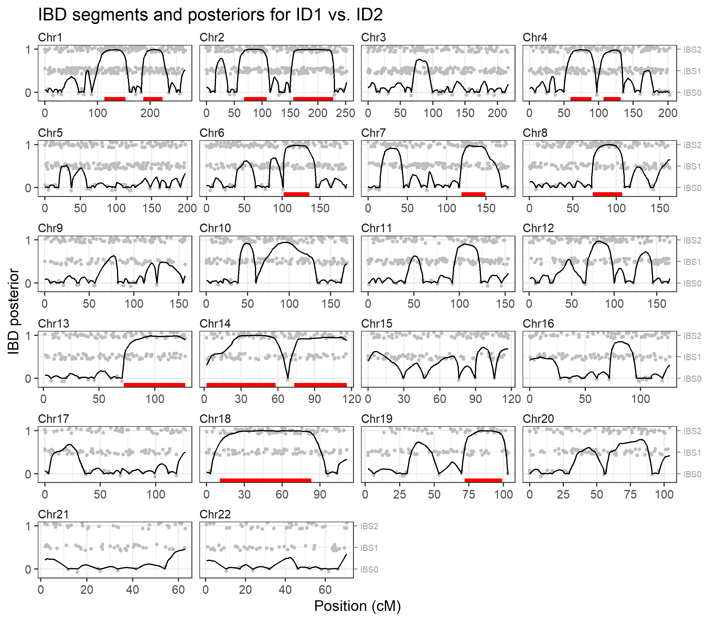
We may also inspect the identified segments as a data frame, showing the start and end positions, and the number of markers in each segment:
ibd$segments
#>    chrom    startCM     endCM   n
#> 1      1 113.000492 153.08623  54
#> 2      1 186.630319 223.39542  46
#> 3      2  67.118524 108.35905  50
#> 4      2 156.120361 227.62362  90
#> 5      4  59.474215  89.85522  41
#> 6      4 106.931772 131.69280  35
#> 7      6 102.041153 136.17734  43
#> 8      7 118.702115 149.11283  38
#> 9      8  72.976430 106.82971  55
#> 10    13  72.049460 127.22724  63
#> 11    14   1.808552  58.07117  67
#> 12    14  73.201009 116.00254  49
#> 13    18  10.592411  83.28443 101
#> 14 19 72.014020 99.15558 34ibdfindr also supports a HMM tailored for full
siblings, with three IBD states 0, 1 and 2. If we apply this to
cousinsDemo it (correctly) reports no IBD2 segments, and in
fact recovers most of the IBD1 segments.
ibdFS = findIBD(cousinsDemo, model = "fullsib")
#> Individuals: ID1, ID2
#> Chromosome type: autosomal
#> Input data: genotypes
#> Dropout probs (supplied): ID1 = 0, ID2 = 0
#> Model: 3-state HMM for full siblings
#> Markers: 3915 input, 0 removed
#> ----
#> Fitting full-sib HMM ...
#>   Optimising `a` conditional on kappa
#>   a = 1.402, loglik = -7750.889
#> ----
#> Finding IBD segments...
#>   IBD0: 31 segments (2798.14 cM, 83.2%)
#>   IBD1: 12 segments (563.93 cM, 16.8%)
#>   IBD2: 0 segments (0.00 cM, 0.0%)
#> Calculating IBD posteriors...
#> Analysis complete in 1.26 secs
Note that the likelihood reported for this model (loglik = -7750.889) is lower here than in the previous analysis (loglik = -7704.393), indicating that the full-sibling model is a worse fit to the data.
The brothersX dataset contains genotypes for two
brothers typed with 246 X-chromosomal SNPs. The analysis below indicates
that they share 3 IBD segments on the X chromosome.
ibdX = findIBD(brothersX)
#> Individuals: ID1, ID2
#> Chromosome type: X (male, male)
#> Input data: genotypes
#> Dropout probs (supplied): ID1 = 0, ID2 = 0
#> Model: 2-state HMM, unilineal relationships
#> Markers: 246 input, 0 removed
#> ----
#> Fitting HMM parameters...
#> Optimising `k1` and `a` jointly; method: L-BFGS-B
#> k1 = 0.502, a = 6.711, loglik = -252.077
#> ----
#> Finding IBD segments...
#> 3 segments (total length: 88.05 cM)
#> Calculating IBD posteriors...
#> Analysis complete in 0.257 secs
plotIBD(ibdX)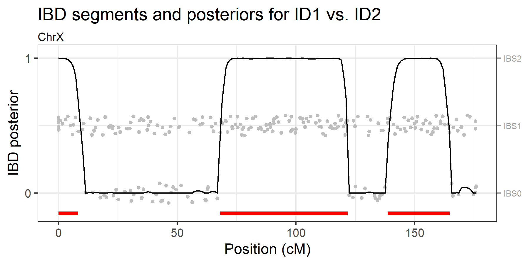 Note that the “fullsib” model is not appropriate in this example, even
if the individuals are full brothers, since the X chromosome is
inherited unilineally in males.
Note that the “fullsib” model is not appropriate in this example, even
if the individuals are full brothers, since the X chromosome is
inherited unilineally in males.
In addition to standard genotype data, ibdfindr also
supports genotype likelihoods (GLs), as typically obtained from low-pass
sequencing data. To exemplify this, we use the built-in dataset
sibsGL containing simulated genotype likelihoods for two
full siblings. The data for each sibling is given in a data frame,
containing base read counts, coverage and genotype likelihoods
(AA, AC, …, TT). Here are the
first three markers for the first sample:
head(sibsGL$data[[1]], 3)
#>       MARKER CHROM     POS A C G T Coverage           AA           AC
#> 1  rs9442372     1 1083324 4 0 7 0       11 9.682262e-15 6.133327e-16
#> 2  rs4648727     1 1844830 1 1 0 0        2 1.337778e-02 1.000000e+00
#> 3 rs10910082     1 2487496 0 0 0 6        6 1.457006e-15 1.457006e-15
#>             AG           AT           CC           CG           CT           GG
#> 1 1.000000e+00 6.133327e-16 1.244374e-24 2.028873e-09 1.244374e-24 2.536566e-07
#> 2 6.711409e-03 6.711409e-03 1.337778e-02 6.711409e-03 6.711409e-03 4.504302e-05
#> 3 1.457006e-15 1.594333e-02 1.457006e-15 1.457006e-15 1.594333e-02 1.457006e-15
#>             GT           TT
#> 1 2.028873e-09 1.244374e-24
#> 2 4.504302e-05 4.504302e-05
#> 3 1.594333e-02 1.000000e+00
(Note that the GLs for each marker are scaled so that the maximum value is 1. This is not a requisite; the values are rescaled internally as part of the processing.)
We first prepare the data with readGL(). This function
accepts either a list of data frames, or a vector of filenames. The SNP
annotation is provided in sibsGL$annot.
gl = readGL(sibsGL$data, sibsGL$annot)We then call findIBD() with the "GL" input
type and the "fullsib" model. The output can be visualised
with plotIBD().
ibdSibs = findIBD(gl, input = "GL", model = "fullsib")
#> Individuals: S1, S2
#> Chromosome type: autosomal
#> Input data: genotype likelihoods
#> Model: 3-state HMM for full siblings
#> Markers: 3930 input, 66 removed, 3864 used
#> Removed markers (categories may overlap):
#>   66 with missing data (S1: 37, S2: 29)
#> ----
#> Fitting full-sib HMM ...
#>   Optimising `a` conditional on kappa
#>   a = 4.148, loglik = -6630.766
#> ----
#> Finding IBD segments...
#>   IBD0: 15 segments (841.79 cM, 25.0%)
#>   IBD1: 43 segments (1521.14 cM, 45.2%)
#>   IBD2: 26 segments (999.14 cM, 29.7%)
#> Calculating IBD posteriors...
#> Analysis complete in 0.462 secsplotIBD(ibdSibs)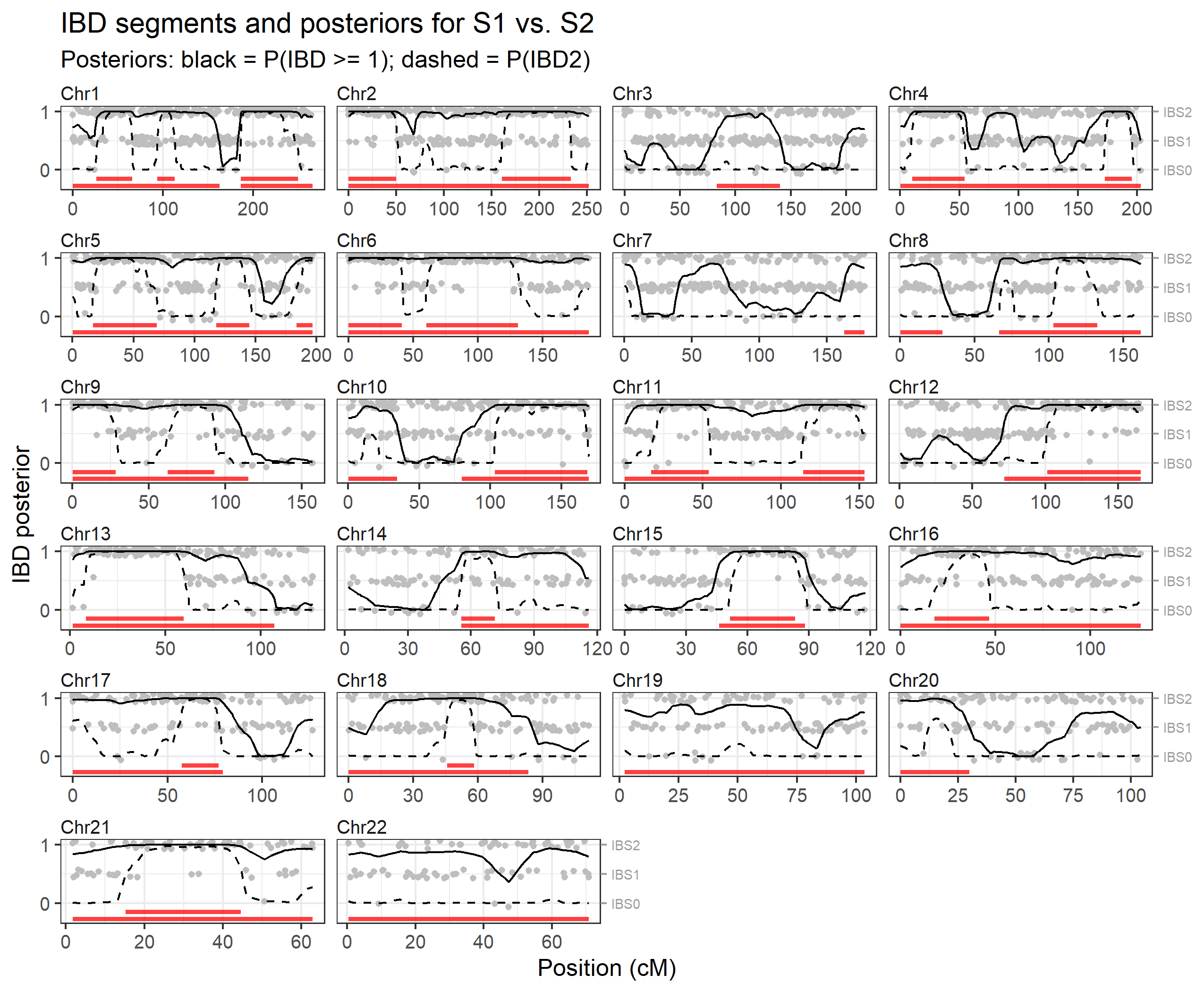
These binaries (installable software) and packages are in development.
They may not be fully stable and should be used with caution. We make no claims about them.