Title:	Statistical Methods for Auditing
Version:	0.7.3
Date:	2025-03-10
Description:	Provides statistical methods for auditing as implemented in JASP for Audit (Derks et al., 2021 <doi:10.21105/joss.02733>). First, the package makes it easy for an auditor to plan a statistical sample, select the sample from the population, and evaluate the misstatement in the sample compliant with international auditing standards. Second, the package provides statistical methods for auditing data, including tests of digit distributions and repeated values. Finally, the package includes methods for auditing algorithms on the aspect of fairness and bias. Next to classical statistical methodology, the package implements Bayesian equivalents of these methods whose statistical underpinnings are described in Derks et al. (2021) <doi:10.1111/ijau.12240>, Derks et al. (2024) <doi:10.2308/AJPT-2021-086>, Derks et al. (2022) <doi:10.31234/osf.io/8nf3e> Derks et al. (2024) <doi:10.31234/osf.io/tgq5z>, and Derks et al. (2025) <doi:10.31234/osf.io/b8tu2>.
Depends:	R (≥ 3.5.0)
Imports:	bde (≥ 1.0.1.1), extraDistr (≥ 1.9.1), ggplot2 (≥ 3.4.2), methods, Rcpp (≥ 0.12.0), RcppParallel (≥ 5.0.1), rstan (≥ 2.26.0), rstantools (≥ 2.2.0), stats, truncdist (≥ 1.0-2)
Suggests:	benford.analysis (≥ 0.1.5), BenfordTests (≥ 1.2.0), BeyondBenford (≥ 1.4), fairness, knitr, MUS (≥ 0.1.6), rmarkdown, samplingbook (≥ 1.2.4), testthat
LinkingTo:	BH (≥ 1.66.0), Rcpp (≥ 0.12.0), RcppEigen (≥ 0.3.3.3.0), RcppParallel (≥ 5.0.1), rstan (≥ 2.26.0), StanHeaders (≥ 2.26.0)
VignetteBuilder:	knitr
URL:	https://koenderks.github.io/jfa/, https://github.com/koenderks/jfa
BugReports:	https://github.com/koenderks/jfa/issues
License:	GPL (≥ 3)
Encoding:	UTF-8
LazyData:	true
NeedsCompilation:	yes
SystemRequirements:	C++17, GNU make
Language:	en-US
RoxygenNote:	7.3.2
Biarch:	true
Packaged:	2025-03-10 09:44:28 UTC; koenderks
Author:	Koen Derks [aut, cre], Lotte Mensink [ctb], Federica Picogna [ctb]
Maintainer:	Koen Derks <k.derks@nyenrode.nl>
Repository:	CRAN
Date/Publication:	2025-03-10 10:10:07 UTC

jfa — Statistical Methods for Auditing

Description

jfa is an R package that provides statistical methods for auditing. The package includes functions for planning, performing, and evaluating an audit sample compliant with international auditing standards, as well as functions for auditing data, such as testing the distribution of leading digits in the data against Benford's law. In addition to offering classical frequentist methods, jfa also provides a straightforward implementation of their Bayesian counterparts.

The functionality of the jfa package and its intended workflow are implemented with a graphical user interface in the Audit module of JASP, a free and open-source software program for statistical analyses.

For documentation on jfa itself, including the manual and user guide for the package, worked examples, and other tutorial information visit the package website.

Author(s)

Please use the citation provided by R when citing this package. A BibTex entry is available from citation('jfa').

See Also

Useful links:

• The vignettes for worked examples.

• The issue page to submit a bug report or feature request.

Examples

# Load the jfa package
library(jfa)

#################################
### Example 1: Audit sampling ###
#################################

# Load the BuildIt population
data('BuildIt')

# Stage 1: Planning
stage1 <- planning(materiality = 0.03, expected = 0.01)
summary(stage1)

# Stage 2: Selection
stage2 <- selection(data = BuildIt, size = stage1,
                    units = 'values', values = 'bookValue',
                    method = 'interval', start = 1)
summary(stage2)

# Stage 3: Execution
sample <- stage2[['sample']]

# Stage 4: Evaluation
stage4 <- evaluation(data = sample, method = 'stringer.binomial',
                     values = 'bookValue', values.audit = 'auditValue')
summary(stage4)

#################################
### Example 2: Data auditing ####
#################################

# Load the sinoForest data set
data('sinoForest')

# Test first digits in the data against Benford's law
digit_test(sinoForest[["value"]], check = "first", reference = "benford")

######################################
### Example 3: Algorithm auditing ####
######################################

# Load the compas data set
data('compas')

# Test algorithmic fairness against Caucasian ethnicity
model_fairness(compas, "Ethnicity", "TwoYrRecidivism", "Predicted",
               privileged = "Caucasian", positive = "yes")

BuildIt Construction Financial Statements

Description

Fictional data from a construction company in the United States, containing 3500 observations identification numbers, book values, and audit values. The audit values are added for illustrative purposes, as these would need to be assessed by the auditor in the execution stage of the audit.

Usage

data(BuildIt)

Format

A data frame with 3500 rows and 3 variables.

ID

unique record identification number.

bookValue

book value in US dollars ($14.47–$2,224.40).

auditValue

true value in US dollars ($14.47–$2,224.40).

References

Derks, K., de Swart, J., Wagenmakers, E.-J., Wille, J., & Wetzels, R. (2021). JASP for audit: Bayesian tools for the auditing practice. Journal of Open Source Software, 6(68), 2733.

Examples

data(BuildIt)

Accounts Receivable

Description

Audit sample obtained from a population of N = 87 accounts receivable, totaling $612,824 in book value (Higgins and Nandram, 2009; Lohr, 2021).

Usage

data(accounts)

Format

A data frame with 20 rows and 3 variables.

account

account number (between 1 - 87)

bookValue

booked value of the account

auditValue

audited (i.e., true) value of the account

References

Higgins, H. N., & Nandram, B. (2009). Monetary unit sampling: Improving estimation of the total audit error Advances in Accounting, 25(2), 174-182. doi:10.1016/j.adiac.2009.06.001

Lohr, S. L. (2021). Sampling: Design and Analysis. CRC press.

Examples

data(accounts)

Legitimacy Audit

Description

Fictional population from a legitimacy audit, containing 4189 records with identification numbers, stratum identifiers, book values, and audit values. The audit values are added for illustrative purposes, as these would need to be assessed by the auditor in the execution stage of the audit.

Usage

data(allowances)

Format

A data frame with 4189 rows and 5 variables.

item

a unique record identification number.

branch

the stratum identifier / branch number.

bookValue

the item book value in US dollars.

auditValue

the item audit (i.e., true) value in US dollars.

times

a sample selection indicator (0 = not in sample).

Examples

data(allowances)

Audit Sampling: Prior Distributions

Description

auditPrior() is used to create a prior distribution for Bayesian audit sampling. The interface allows a complete customization of the prior distribution as well as a formal translation of pre-existing audit information into a prior distribution. The function returns an object of class jfaPrior that can be used in the planning() and evaluation() functions via their prior argument. Objects with class jfaPrior can be further inspected via associated summary() and plot() methods.

Usage

auditPrior(
  method = c(
    "default", "param", "strict", "impartial", "hyp",
    "arm", "bram", "sample", "power", "nonparam"
  ),
  likelihood = c(
    "poisson", "binomial", "hypergeometric",
    "normal", "uniform", "cauchy", "t", "chisq",
    "exponential"
  ),
  N.units = NULL,
  alpha = NULL,
  beta = NULL,
  materiality = NULL,
  expected = 0,
  ir = NULL,
  cr = NULL,
  ub = NULL,
  p.hmin = NULL,
  x = NULL,
  n = NULL,
  delta = NULL,
  samples = NULL,
  conf.level = 0.95
)

Arguments

Details

To perform Bayesian audit sampling you must assign a prior distribution to the parameter in the model, i.e., the population misstatement \theta. The prior distribution can incorporate pre-existing audit information about \theta into the analysis, which consequently allows for a more efficient or more accurate estimates. The default priors used by jfa are indifferent towards the possible values of \theta, while still being proper. Note that the default prior distributions are a conservative choice of prior since they, in most cases, assume all possible misstatement to be equally likely before seeing a data sample. It is recommended to construct an informed prior distribution based on pre-existing audit information when possible.

This section elaborates on the available input options for the method argument.

• default: This method produces a gamma(1, 1), beta(1, 1), beta-binomial(N, 1, 1), normal(0.5, 1000) , cauchy(0, 1000), student-t(1), or chi-squared(1) prior distribution. These prior distributions are mostly indifferent about the possible values of the misstatement.

• param: This method produces a custom gamma(alpha, beta), beta(alpha, beta), beta-binomial(N, alpha, beta) prior distribution, normal(alpha, beta), cauchy(alpha, beta), student-t(alpha), or chi-squared(alpha). The alpha and beta parameters must be set using alpha and beta.

• strict: This method produces an improper gamma(1, 0), beta(1, 0), or beta-binomial(N, 1, 0) prior distribution. These prior distributions match sample sizes and upper limits from classical methods and can be used to emulate classical results.

• impartial: This method produces an impartial prior distribution. These prior distributions assume that tolerable misstatement (\theta < materiality) and intolerable misstatement (\theta > materiality) are equally likely.

• hyp: This method translates an assessment of the prior probability for tolerable misstatement (\theta < materiality) to a prior distribution.

• arm: This method translates an assessment of inherent risk and internal control risk to a prior distribution.

• bram: This method translates an assessment of the expected most likely error and x-% upper bound to a prior distribution.

• sample: This method translates the outcome of an earlier sample to a prior distribution.

• power: This method translates and weighs the outcome of an earlier sample to a prior distribution (i.e., a power prior).

• nonparam: This method takes a vector of samples from the prior distribution (via samples) and constructs a bounded density (between 0 and 1) on the basis of these samples to act as the prior.

This section elaborates on the available input options for the likelihood argument and the corresponding conjugate prior distributions used by jfa.

• poisson: The Poisson distribution is an approximation of the binomial distribution. The Poisson distribution is defined as:

  f(\theta, n) = \frac{\lambda^\theta e^{-\lambda}}{\theta!}

  . The conjugate gamma(\alpha, \beta) prior has probability density function:

  p(\theta; \alpha, \beta) = \frac{\beta^\alpha \theta^{\alpha - 1} e^{-\beta \theta}}{\Gamma(\alpha)}

  .

• binomial: The binomial distribution is an approximation of the hypergeometric distribution. The binomial distribution is defined as:

  f(\theta, n, x) = {n \choose x} \theta^x (1 - \theta)^{n - x}

  . The conjugate beta(\alpha, \beta) prior has probability density function:

  p(\theta; \alpha, \beta) = \frac{1}{B(\alpha, \beta)} \theta^{\alpha - 1} (1 - \theta)^{\beta - 1}

  .

• hypergeometric: The hypergeometric distribution is defined as:

  f(x, n, K, N) = \frac{{K \choose x} {N - K \choose n - x}} {{N \choose n}}

  . The conjugate beta-binomial(\alpha, \beta) prior (Dyer and Pierce, 1993) has probability mass function:

  f(x, n, \alpha, \beta) = {n \choose x} \frac{B(x + \alpha, n - x + \beta)}{B(\alpha, \beta)}

  .

Value

An object of class jfaPrior containing:

Author(s)

Koen Derks, k.derks@nyenrode.nl

References

Derks, K., de Swart, J., van Batenburg, P., Wagenmakers, E.-J., & Wetzels, R. (2021). Priors in a Bayesian audit: How integration of existing information into the prior distribution can improve audit transparency and efficiency. International Journal of Auditing, 25(3), 621-636. doi:10.1111/ijau.12240

Derks, K., de Swart, J., Wagenmakers, E.-J., Wille, J., & Wetzels, R. (2021). JASP for audit: Bayesian tools for the auditing practice. Journal of Open Source Software, 6(68), 2733. doi:10.21105/joss.02733

Derks, K., de Swart, J., Wagenmakers, E.-J., & Wetzels, R. (2022). An impartial Bayesian hypothesis test for audit sampling. PsyArXiv. doi:10.31234/osf.io/8nf3e

See Also

planning selection evaluation

Examples

# Default beta prior
auditPrior(likelihood = "binomial")

# Impartial prior
auditPrior(method = "impartial", materiality = 0.05)

# Non-conjugate prior
auditPrior(method = "param", likelihood = "normal", alpha = 0, beta = 0.1)

Benchmark Analysis of Sales Versus Cost of Sales

Description

Fictional data from a benchmark analysis comparing industry sales versus the industry cost of sales.

Usage

data(benchmark)

Format

A data frame with 100 rows and 2 variables.

sales

book value in US dollars ($100,187,432–$398,280,933).

costofsales

true value in US dollars ($71,193,639–$309,475,784).

References

Derks, K., de Swart, J., van Batenburg, P., Wagenmakers, E.-J., & Wetzels, R. (2021). Priors in a Bayesian audit: How integration of existing information into the prior distribution can improve audit transparency and efficiency. International Journal of Auditing, 25(3), 621-636. doi:10.1111/ijau.12240

Examples

data(benchmark)

Carrier Company Financial Statements

Description

Fictional data from a carrier company in Europe, containing 202 ledger items across 10 company entities.

Usage

data(carrier)

Format

A data frame with 202 rows and 12 variables.

description

description of the ledger item.

entity1

recorded values for entity 1, in US dollars.

entity2

recorded values for entity 2, in US dollars.

entity3

recorded values for entity 3, in US dollars.

entity4

recorded values for entity 4, in US dollars.

entity5

recorded values for entity 5, in US dollars.

entity6

recorded values for entity 6, in US dollars.

entity7

recorded values for entity 7, in US dollars.

entity8

recorded values for entity 8, in US dollars.

entity9

recorded values for entity 9, in US dollars.

entity10

recorded values for entity 10, in US dollars.

total

total value, in US dollars.

Source

https://medium.com/towards-data-science/data-driven-audit-1-automated-sampling-using-python-52e83347add5

Examples

data(carrier)

COMPAS Recidivism Prediction

Description

This data was used to predict recidivism (whether a criminal will reoffend or not) in the USA.

Usage

data(compas)

Format

A data frame with 100 rows and 2 variables.

TwoYrRecidivism

yes/no for recidivism or no recidivism.

AgeAboveFourtyFive

yes/no for age above 45 years or not

AgeBelowTwentyFive

yes/no for age below 25 years or not

Gender

female/male for gender

Misdemeanor

yes/no for having recorded misdemeanor(s) or not

Ethnicity

Caucasian, African American, Asian, Hispanic, Native American or Other

Predicted

yes/no, predicted values for recidivism

References

https://www.kaggle.com/danofer/compass https://cran.r-project.org/package=fairness

Examples

data(compas)

Data Auditing: Digit Distribution Test

Description

This function extracts and performs a test of the distribution of (leading) digits in a vector against a reference distribution. By default, the distribution of leading digits is checked against Benford's law.

Usage

digit_test(
  x,
  check = c("first", "last", "firsttwo", "lasttwo"),
  reference = "benford",
  conf.level = 0.95,
  prior = FALSE
)

Arguments

Details

Benford's law is defined as p(d) = log10(1/d). The uniform distribution is defined as p(d) = 1/d.

Value

An object of class jfaDistr containing:

Author(s)

Koen Derks, k.derks@nyenrode.nl

References

Benford, F. (1938). The law of anomalous numbers. In Proceedings of the American Philosophical Society, 551-572.

See Also

repeated_test

Examples

set.seed(1)
x <- rnorm(100)

# First digit analysis against Benford's law
digit_test(x, check = "first", reference = "benford")

# Bayesian first digit analysis against Benford's law
digit_test(x, check = "first", reference = "benford", prior = TRUE)

# Last digit analysis against the uniform distribution
digit_test(x, check = "last", reference = "uniform")

# Bayesian last digit analysis against the uniform distribution
digit_test(x, check = "last", reference = "uniform", prior = TRUE)

# First digit analysis against a custom distribution
digit_test(x, check = "last", reference = 1:9)

# Bayesian first digit analysis against a custom distribution
digit_test(x, check = "last", reference = 1:9, prior = TRUE)

Audit Sampling: Evaluation

Description

evaluation() is used to perform statistical inference about the misstatement in a population after auditing a statistical sample. It allows specification of statistical requirements for the sample with respect to the performance materiality or the precision. The function returns an object of class jfaEvaluation that can be used with associated summary() and plot() methods.

Usage

evaluation(
  materiality = NULL,
  method = c(
    "poisson", "binomial", "hypergeometric",
    "inflated.poisson", "hurdle.beta",
    "stringer.poisson", "stringer.binomial", "stringer.hypergeometric",
    "stringer.meikle", "stringer.lta", "stringer.pvz", "stringer",
    "rohrbach", "moment", "coxsnell", "mpu", "pps",
    "direct", "difference", "quotient", "regression"
  ),
  alternative = c("less", "two.sided", "greater"),
  conf.level = 0.95,
  data = NULL,
  values = NULL,
  values.audit = NULL,
  strata = NULL,
  times = NULL,
  x = NULL,
  n = NULL,
  N.units = NULL,
  N.items = NULL,
  pooling = c("none", "complete", "partial"),
  prior = FALSE
)

Arguments

Details

This section lists the available options for the method argument.

• poisson: Evaluates the sample with the Poisson distribution. If combined with prior = TRUE, performs Bayesian evaluation using a gamma prior.

• binomial: Evaluates the sample with the binomial distribution. If combined with prior = TRUE, performs Bayesian evaluation using a beta prior.

• hypergeometric: Evaluates the sample with the hypergeometric distribution. If combined with prior = TRUE, performs Bayesian evaluation using a beta-binomial prior.

• inflated.poisson: Inflated Poisson model incorporating the explicit probability of misstatement being zero. If prior = TRUE, performs Bayesian evaluation using a beta prior.

• hurdle.beta: Hurdle beta model incorporating the explicit probability of a taint being zero, one, or in between. If prior = TRUE, this setup performs Bayesian evaluation using a beta prior.

• stringer.poisson: Evaluates the sample with the Stringer bound using the Poisson distribution.

• stringer.binomial: Evaluates the sample with the Stringer bound using the binomial distribution (Stringer, 1963).

• stringer.hypergeometric: Evaluates the sample with the Stringer bound using the hypergeometric distribution.

• stringer.meikle: Evaluates the sample using the Stringer bound with Meikle's correction for understatements (Meikle, 1972).

• stringer.lta: Evaluates the sample using the Stringer bound with LTA correction for understatements (Leslie, Teitlebaum, and Anderson, 1979).

• stringer.pvz: Evaluates the sample using the Stringer bound with Pap and van Zuijlen's correction for understatements (Pap and van Zuijlen, 1996).

• rohrbach: Evaluates the sample using Rohrbach's augmented variance bound (Rohrbach, 1993).

• moment: Evaluates the sample using the modified moment bound (Dworin and Grimlund, 1984).

• coxsnell: Evaluates the sample using the Cox and Snell bound (Cox and Snell, 1979).

• mpu: Evaluates the sample with the mean-per-unit estimator using the Normal distribution.

• pps: Evaluates the sample with the proportional-to-size estimator using the Student-t distribution.

• direct: Evaluates the sample using the direct estimator (Touw and Hoogduin, 2011).

• difference: Evaluates the sample using the difference estimator (Touw and Hoogduin, 2011).

• quotient: Evaluates the sample using the quotient estimator (Touw and Hoogduin, 2011).

• regression: Evaluates the sample using the regression estimator (Touw and Hoogduin, 2011).

Value

An object of class jfaEvaluation containing:

Author(s)

Koen Derks, k.derks@nyenrode.nl

References

Cox, D. and Snell, E. (1979). On sampling and the estimation of rare errors. Biometrika, 66(1), 125-132. doi:10.1093/biomet/66.1.125.

Derks, K., de Swart, J., van Batenburg, P., Wagenmakers, E.-J., & Wetzels, R. (2021). Priors in a Bayesian audit: How integration of existing information into the prior distribution can improve audit transparency and efficiency. International Journal of Auditing, 25(3), 621-636. doi:10.1111/ijau.12240

Derks, K., de Swart, J., Wagenmakers, E.-J., Wille, J., & Wetzels, R. (2021). JASP for audit: Bayesian tools for the auditing practice. Journal of Open Source Software, 6(68), 2733. doi:10.21105/joss.02733

Derks, K., de Swart, J., Wagenmakers, E.-J., & Wetzels, R. (2024). The Bayesian approach to audit evidence: Quantifying statistical evidence using the Bayes factor. Auditing: A Journal of Practice & Theory. doi:10.2308/AJPT-2021-086

Derks, K., de Swart, J., Wagenmakers, E.-J., & Wetzels, R. (2022). An impartial Bayesian hypothesis test for audit sampling. PsyArXiv. doi:10.31234/osf.io/8nf3e

Derks, K., de Swart, J., Wagenmakers, E.-J., & Wetzels, R. (2022). Bayesian generalized linear modeling for audit sampling: How to incorporate audit information into the statistical model. PsyArXiv. doi:10.31234/osf.io/byj2a

Dworin, L. D. and Grimlund, R. A. (1984). Dollar-unit sampling for accounts receivable and inventory. The Accounting Review, 59(2), 218-241. https://www.jstor.org/stable/247296

Leslie, D. A., Teitlebaum, A. D., & Anderson, R. J. (1979). Dollar-unit Sampling: A Practical Guide for Auditors. Copp Clark Pitman; Belmont, CA. ISBN: 9780773042780.

Meikle, G. R. (1972). Statistical Sampling in an Audit Context. Canadian Institute of Chartered Accountants.

Pap, G., and van Zuijlen, M. C. (1996). On the asymptotic behavior of the Stringer bound. Statistica Neerlandica, 50(3), 367-389. doi:10.1111/j.1467-9574.1996.tb01503.x.

Rohrbach, K. J. (1993). Variance augmentation to achieve nominal coverage probability in sampling from audit populations. Auditing, 12(2), 79.

Stringer, K. W. (1963). Practical aspects of statistical sampling in auditing. In Proceedings of the Business and Economic Statistics Section (pp. 405-411). American Statistical Association.

Touw, P., and Hoogduin, L. (2011). Statistiek voor Audit en Controlling. Boom uitgevers Amsterdam.

See Also

auditPrior planning selection

Examples

# Using summary statistics
evaluation(materiality = 0.05, x = 0, n = 100) # Non-stratified
evaluation(materiality = 0.05, x = c(2, 1, 0), n = c(50, 70, 40)) # Stratified

# Using data
data("BuildIt")
BuildIt$inSample <- c(rep(1, 100), rep(0, 3400))
levs <- c("low", "medium", "high")
BuildIt$stratum <- factor(c(levs[3], levs[2], rep(levs, times = 1166)))
sample <- subset(BuildIt, BuildIt$inSample == 1)

# Non-stratified evaluation
evaluation(
  materiality = 0.05, data = sample,
  values = "bookValue", values.audit = "auditValue"
)
# Stratified evaluation
evaluation(
  materiality = 0.05, data = sample, values = "bookValue",
  values.audit = "auditValue", strata = "stratum"
)

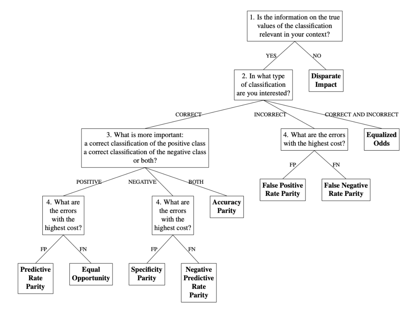
Algorithm Auditing: Fairness Measures Selection

Description

This function aims to provide a fairness measure tailored to a specific context and dataset by answering the questions in the developed decision-making workflow. The questions within the decision-making workflow are based on observable data characteristics, the properties of fairness measures and the information required for their calculation. However, these questions are posed to the user in an easily understandable manner, requiring no statistical background or in-depth knowledge of the fairness measures. Obtainable fairness measures include Disparate Impact, Equalized Odds, Predictive Rate Parity, Equal Opportunity, Specificity Parity, Negative Predictive Rate Parity, Accuracy Parity, False Positive Rate Parity and False Negative Rate Parity. The function returns an object of class jfaFairnessSelection that can be used with associated print() and plot() methods.

Usage

fairness_selection(
  q1 = NULL,
  q2 = NULL,
  q3 = NULL,
  q4 = NULL
)

Arguments

Details

Several fairness measures can be used to assess the fairness of AI-predicted classifications. These include:

• Disparate Impact. See Friedler et al. (2019), Feldman et al. (2015), Castelnovo et al. (2022) for a more detailed explanation of this measure.

• Equalized Odds. See Hardt et al. (2016), Verma et al. (2018) and Picogna et al. (2025) for a more detailed explanation of this measure.

• False Positive Rate Parity. See Castelnovo et al. (2022) (under the name Predictive Equality), Verma et al. (2018) and Picogna et al. (2025) for a more detailed explanation of this measure.

• False Negative Rate Parity. See Castelnovo et al. (2022) (under the name Equality of Opportunity), Verma et al. (2018) and and Picogna et al. (2025) for a more detailed explanation of this measure.

• Predictive Rate Parity. See Castelnovo et al. (2022) (under the name Predictive Parity) and Picogna et al. (2025) for a more detailed explanation of this measure.

• Equal Opportunity. See Hardt et al. (2016), Friedler et al. (2019), Verma et al. (2018) and Picogna et al. (2025) for a more detailed explanation of this measure.

• Specificity Parity. See Friedler et al. (2019), Verma et al. (2018) and Picogna et al. (2025) for a more detailed explanation of this measure.

• Negative Predictive Value Parity. See Verma et al. (2018) and Picogna et al. (2025) for a more detailed explanation of this measure.

• Accuracy Parity. See Friedler et al. (2019) and Picogna et al. (2025) for a more detailed explanation of this measure.

The fairness decision-making workflow below aids in choosing which fairness measure is appropriate for the situation at hand (Picogna et al., 2025).

Value

An object of class jfaFairnessSelection containing:

Author(s)

Federica Picogna, f.picogna@nyenrode.nl

References

Castelnovo, A., Crupi, R., Greco, G. et al. (2022). A clarification of the nuances in the fairness metrics landscape. In Sci Rep 12, 4209. doi:10.1038/s41598-022-07939-1

Feldman, M., Friedler, S. A., Moeller, J., Scheidegger, C., & Venkatasubramanian, S. (2015). Certifying and removing disparate impact. In Proceedings of the 21th ACM SIGKDD International Conference on Knowledge Discovery and Data Mining. doi:10.1145/2783258.2783311

Friedler, S. A., Scheidegger, C., Venkatasubramanian, S., Choudhary, S., Hamilton, E. P., & Roth, D. (2019). A comparative study of fairness-enhancing interventions in machine learning. In Proceedings of the Conference on Fairness, Accountability, and Transparency. doi:10.1145/3287560.3287589

Hardt M. , Price E., Srebro N. (2016). Equality of opportunity in supervised learning. In Advances in neural information processing systems, 29. doi:10.48550/arXiv.1610.02413

Picogna, F., de Swart, J., Kaya, H., & Wetzels, R. (2025). How to choose a fairness measure: A decision-making workflow for auditors. doi:10.31219/osf.io/cpxmf_v1

Verma S., Rubin J. (2018). Fairness definitions explained. In Proceedings of the international workshop on software fairness, 1–7. doi:10.1145/3194770.3194776

Examples

# Workflow leading to predictive rate parity
fairness_selection(q1 = 1, q2 = 1, q3 = 1, q4 = 1)

Methods for jfa objects

Description

Methods defined for objects returned from the auditPrior, planning, selection, and evaluation functions.

Usage

## S3 method for class 'jfaPrior'
print(x, ...)

## S3 method for class 'summary.jfaPrior'
print(x, digits = getOption("digits"), ...)

## S3 method for class 'jfaPrior'
summary(object, digits = getOption("digits"), ...)

## S3 method for class 'jfaPrior'
predict(object, n, cumulative = FALSE, ...)

## S3 method for class 'jfaPredict'
print(x, ...)

## S3 method for class 'jfaPrior'
plot(x, ...)

## S3 method for class 'jfaPredict'
plot(x, ...)

## S3 method for class 'jfaPosterior'
print(x, ...)

## S3 method for class 'summary.jfaPosterior'
print(x, digits = getOption("digits"), ...)

## S3 method for class 'jfaPosterior'
summary(object, digits = getOption("digits"), ...)

## S3 method for class 'jfaPosterior'
predict(object, n, cumulative = FALSE, ...)

## S3 method for class 'jfaPosterior'
plot(x, ...)

## S3 method for class 'jfaPlanning'
print(x, ...)

## S3 method for class 'summary.jfaPlanning'
print(x, digits = getOption("digits"), ...)

## S3 method for class 'jfaPlanning'
summary(object, digits = getOption("digits"), ...)

## S3 method for class 'jfaPlanning'
plot(x, ...)

## S3 method for class 'jfaSelection'
print(x, ...)

## S3 method for class 'summary.jfaSelection'
print(x, digits = getOption("digits"), ...)

## S3 method for class 'jfaSelection'
summary(object, digits = getOption("digits"), ...)

## S3 method for class 'jfaEvaluation'
print(x, digits = getOption("digits"), ...)

## S3 method for class 'summary.jfaEvaluation'
print(x, digits = getOption("digits"), ...)

## S3 method for class 'jfaEvaluation'
summary(object, digits = getOption("digits"), ...)

## S3 method for class 'jfaEvaluation'
plot(x, type = c("estimates", "posterior", "sequential"), ...)

## S3 method for class 'jfaDistr'
print(x, digits = getOption("digits"), ...)

## S3 method for class 'summary.jfaDistr'
print(x, digits = getOption("digits"), ...)

## S3 method for class 'jfaDistr'
summary(object, digits = getOption("digits"), ...)

## S3 method for class 'jfaDistr'
plot(x, type = c("estimates", "robustness", "sequential"), ...)

## S3 method for class 'jfaRv'
print(x, digits = getOption("digits"), ...)

## S3 method for class 'jfaRv'
plot(x, ...)

## S3 method for class 'jfaFairness'
print(x, digits = getOption("digits"), ...)

## S3 method for class 'summary.jfaFairness'
print(x, digits = getOption("digits"), ...)

## S3 method for class 'jfaFairness'
summary(object, digits = getOption("digits"), ...)

## S3 method for class 'jfaFairness'
plot(x, type = c("estimates", "posterior", "robustness", "sequential"), ...)

## S3 method for class 'jfaFairnessSelection'
print(x, ...)

## S3 method for class 'jfaFairnessSelection'
plot(x, ...)

Arguments

Value

The summary methods return a data.frame which contains the input and output.

The print methods simply print and return nothing.

Algorithm Auditing: Fairness Metrics and Parity

Description

This function aims to assess fairness in algorithmic decision-making systems by computing and testing the equality of one of several model-agnostic fairness metrics between protected classes. The metrics are computed based on a set of true labels and the predictions of an algorithm. The ratio of these metrics between any unprivileged protected class and the privileged protected class is called parity. This measure can quantify potential fairness or discrimination in the algorithms predictions. Available parity metrics include predictive rate parity, proportional parity, accuracy parity, false negative rate parity, false positive rate parity, true positive rate parity, negative predictive value parity, specificity parity, and demographic parity. The function returns an object of class jfaFairness that can be used with associated summary() and plot() methods.

Usage

model_fairness(
  data,
  protected,
  target,
  predictions,
  privileged = NULL,
  positive = NULL,
  metric = c(
    "prp", "pp", "ap", "fnrp", "fprp",
    "tprp", "npvp", "sp", "dp", "eo"
  ),
  alternative = c("two.sided", "less", "greater"),
  conf.level = 0.95,
  prior = FALSE
)

Arguments

Details

The following model-agnostic fairness metrics are computed based on the confusion matrix for each protected class, using the true positives (TP), false positives (FP), true negative (TN) and false negatives (FN). See Pessach & Shmueli (2022) for a more detailed explanation of the individual metrics. The equality of metrics across groups is done according to the methodology described in Fisher (1970) and Jamil et al. (2017).

• Predictive rate parity (prp): calculated as TP / (TP + FP), its ratio quantifies whether the predictive rate is equal across protected classes.

• Proportional parity (pp): calculated as (TP + FP) / (TP + FP + TN + FN), its ratio quantifies whether the positive prediction rate is equal across protected classes.

• Accuracy parity (ap): calculated as (TP + TN) / (TP + FP + TN + FN), quantifies whether the accuracy is the same across groups.

• False negative rate parity (fnrp): calculated as FN / (TP + FN), quantifies whether the false negative rate is the same across groups.

• False positive rate parity (fprp): calculated as FP / (TN + FP), quantifies whether the false positive rate is the same across groups.

• True positive rate parity (tprp, also known as equal opportunity): calculated as TP / (TP + FN), quantifies whether the true positive rate is the same across groups.

• Negative predictive value parity (npvp): calculated as TN / (TN + FN), quantifies whether the negative predictive value is equal across groups.

• Specificity parity (sp): calculated as TN / (TN + FP), quantifies whether the true positive rate is the same across groups.

• Demographic parity (dp): calculated as TP + FP, quantifies whether the positive predictions are equal across groups.

• Equalized odds (eo): calculated as a combination of the true positive rate and the false positive rate, quantifies whether the true positive rate and, simultaneously, the false positive rate are the same across groups

Note that, in an audit context, not all fairness measures are equally appropriate in all situations. The fairness tree below aids in choosing which fairness measure is appropriate for the situation at hand (Picogna et al., 2025).

Value

An object of class jfaFairness containing:

Author(s)

Koen Derks, k.derks@nyenrode.nl

References

Calders, T., & Verwer, S. (2010). Three naive Bayes approaches for discrimination-free classification. In Data Mining and Knowledge Discovery. Springer Science and Business Media LLC. doi:10.1007/s10618-010-0190-x

Chouldechova, A. (2017). Fair prediction with disparate impact: A study of bias in recidivism prediction instruments. In Big Data. Mary Ann Liebert Inc. doi:10.1089/big.2016.0047

Feldman, M., Friedler, S. A., Moeller, J., Scheidegger, C., & Venkatasubramanian, S. (2015). Certifying and removing disparate impact. In Proceedings of the 21th ACM SIGKDD International Conference on Knowledge Discovery and Data Mining. doi:10.1145/2783258.2783311

Friedler, S. A., Scheidegger, C., Venkatasubramanian, S., Choudhary, S., Hamilton, E. P., & Roth, D. (2019). A comparative study of fairness-enhancing interventions in machine learning. In Proceedings of the Conference on Fairness, Accountability, and Transparency. doi:10.1145/3287560.3287589

Fisher, R. A. (1970). Statistical Methods for Research Workers. Oliver & Boyd.

Jamil, T., Ly, A., Morey, R. D., Love, J., Marsman, M., & Wagenmakers, E. J. (2017). Default "Gunel and Dickey" Bayes factors for contingency tables. Behavior Research Methods, 49, 638-652. doi:10.3758/s13428-016-0739-8

Pessach, D. & Shmueli, E. (2022). A review on fairness in machine learning. ACM Computing Surveys, 55(3), 1-44. doi:10.1145/3494672

Picogna, F., de Swart, J., Kaya, H., & Wetzels, R. (2025). How to choose a fairness measure: A decision-making workflow for auditors. doi:10.31219/osf.io/cpxmf_v1

Zafar, M. B., Valera, I., Gomez Rodriguez, M., & Gummadi, K. P. (2017). Fairness beyond disparate treatment & disparate impact. In Proceedings of the 26th International Conference on World Wide Web. doi:10.1145/3038912.3052660

Examples

# Frequentist test of specificy parity
model_fairness(
  data = compas,
  protected = "Gender",
  target = "TwoYrRecidivism",
  predictions = "Predicted",
  privileged = "Male",
  positive = "yes",
  metric = "sp"
)

Audit Sampling: Planning

Description

planning() is used to calculate a minimum sample size for audit samples. It allows specification of statistical requirements for the sample with respect to the performance materiality or the precision. The function returns an object of class jfaPlanning that can be used with associated summary() and plot() methods.

Usage

planning(
  materiality = NULL,
  min.precision = NULL,
  expected = 0,
  likelihood = c("poisson", "binomial", "hypergeometric"),
  conf.level = 0.95,
  N.units = NULL,
  by = 1,
  max = 5000,
  prior = FALSE
)

Arguments

Details

This section elaborates on the available input options for the likelihood argument and the corresponding conjugate prior distributions used by jfa.

• poisson: The Poisson distribution is an approximation of the binomial distribution. The Poisson distribution is defined as:

  f(\theta, n) = \frac{\lambda^\theta e^{-\lambda}}{\theta!}

  . The conjugate gamma(\alpha, \beta) prior has probability density function:

  p(\theta; \alpha, \beta) = \frac{\beta^\alpha \theta^{\alpha - 1} e^{-\beta \theta}}{\Gamma(\alpha)}

  .

• binomial: The binomial distribution is an approximation of the hypergeometric distribution. The binomial distribution is defined as:

  f(\theta, n, x) = {n \choose x} \theta^x (1 - \theta)^{n - x}

  . The conjugate beta(\alpha, \beta) prior has probability density function:

  p(\theta; \alpha, \beta) = \frac{1}{B(\alpha, \beta)} \theta^{\alpha - 1} (1 - \theta)^{\beta - 1}

  .

• hypergeometric: The hypergeometric distribution is defined as:

  f(x, n, K, N) = \frac{{K \choose x} {N - K \choose n - x}} {{N \choose n}}

  . The conjugate beta-binomial(\alpha, \beta) prior (Dyer and Pierce, 1993) has probability mass function:

  f(x, n, \alpha, \beta) = {n \choose x} \frac{B(x + \alpha, n - x + \beta)}{B(\alpha, \beta)}

  .

Value

An object of class jfaPlanning containing:

Author(s)

Koen Derks, k.derks@nyenrode.nl

References

Derks, K., de Swart, J., van Batenburg, P., Wagenmakers, E.-J., & Wetzels, R. (2021). Priors in a Bayesian audit: How integration of existing information into the prior distribution can improve audit transparency and efficiency. International Journal of Auditing, 25(3), 621-636. doi:10.1111/ijau.12240

Derks, K., de Swart, J., Wagenmakers, E.-J., Wille, J., & Wetzels, R. (2021). JASP for audit: Bayesian tools for the auditing practice. Journal of Open Source Software, 6(68), 2733. doi:10.21105/joss.02733

Dyer, D. and Pierce, R.L. (1993). On the choice of the prior distribution in hypergeometric sampling. Communications in Statistics - Theory and Methods, 22(8), 2125-2146. doi:10.1080/03610929308831139

See Also

auditPrior selection evaluation

Examples

# Classical planning
planning(materiality = 0.03, expected = 0)

# Classical two-stage planning
planning(materiality = 0.03, expected = c(1, 0))

# Bayesian planning using a default prior
planning(materiality = 0.03, prior = TRUE)

# Bayesian planning using a custom prior
prior <- auditPrior(method = "impartial", materiality = 0.05)
planning(materiality = 0.05, prior = prior)

Data Auditing: Repeated Values Test

Description

This function analyzes the frequency with which values get repeated within a set of numbers. Unlike Benford's law, and its generalizations, this approach examines the entire number at once, not only the first or last digit(s).

Usage

repeated_test(
  x,
  check = c("last", "lasttwo", "all"),
  method = c("af", "entropy"),
  samples = 2000
)

Arguments

Details

To determine whether the data show an excessive amount of bunching, the null hypothesis that x does not contain an unexpected amount of repeated values is tested against the alternative hypothesis that x has more repeated values than expected. The statistic can either be the average frequency (AF = sum(f_i^2)/sum(f_i)) of the data or the entropy (E = - sum(p_i * log(p_i)), with p_i=f_i/n) of the data. Average frequency and entropy are highly correlated, but the average frequency is often more interpretable. For example, an average frequency of 2.5 means that, on average, your observations contain a value that appears 2.5 times in the data set.To quantify what is expected, this test requires the assumption that the integer portions of the numbers are not associated with their decimal portions.

Value

An object of class jfaRv containing:

Author(s)

Koen Derks, k.derks@nyenrode.nl

References

Simohnsohn, U. (2019, May 25). Number-Bunching: A New Tool for Forensic Data Analysis. Retrieved from https://datacolada.org/77.

See Also

digit_test

Examples

set.seed(1)
x <- rnorm(50)

# Repeated values analysis shuffling last digit
repeated_test(x, check = "last", method = "af", samples = 2000)

Retailer Group Audit

Description

Sample outcomes summarized per branch from an audit of a retail company consisting of 20 branches.

Usage

data(retailer)

Format

A data frame with 20 rows and 5 variables.

stratum

branch/stratum number.

items

total number of items in each branch.

samples

number of items in sample per branch.

errors

number of errors in sample per branch.

Source

Derks, K., de Swart, J., & Wetzels, R. (2022). Een Bayesiaanse blik op gestratificeerde steekproeven heeft voordelen voor de auditor. Maandblad voor Accountancy en Bedrijfseconomie, 96(1/2), 37-46. doi:10.5117/mab.96.78836

Examples

data(retailer)

Factory Workers' use of Hand Sanitizer

Description

Data from a study on factory workers' use of hand sanitizer. Sanitizer use was measured to a 100th of a gram.

Usage

data(sanitizer)

Format

A data frame with 1600 rows and 1 variable.

Source

http://datacolada.org/appendix/74/

References

[Retracted] Li, M., Sun, Y., & Chen, H. (2019). The decoy effect as a nudge: Boosting hand hygiene with a worse option. Psychological Science, 30, 139–149.

Examples

data(sanitizer)

Audit Sampling: Selection

Description

selection() is used to perform statistical selection of audit samples. It offers flexible implementations of the most common audit sampling algorithms for attributes sampling and monetary unit sampling. The function returns an object of class jfaSelection that can be used with the associated summary() method.

Usage

selection(
  data,
  size,
  units = c("items", "values"),
  method = c("interval", "cell", "random", "sieve"),
  values = NULL,
  order = NULL,
  decreasing = FALSE,
  randomize = FALSE,
  replace = FALSE,
  start = 1
)

Arguments

Details

This section elaborates on the possible options for the units argument:

• items: In attributes sampling each item in the population is a sampling unit. An item with a book value of $5000 is therefore equally likely to be selected as an item with a book value of $500.

• values: In monetary unit sampling each monetary unit in the population is a sampling unit. An item with a book value of $5000 is therefore ten times more likely to be selected as an item with a book value of $500.

This section elaborates on the possible options for the method argument:

• interval: In fixed interval sampling the sampling units are divided into a number of equally large intervals. In each interval, a single sampling unit is selected according to a fixed starting point (specified by start).

• cell: In cell sampling the sampling units in the population are divided into a number (equal to the sample size) of equally large intervals. In each interval, a single sampling unit is selected randomly.

• random: In random sampling all sampling units are drawn with equal probability.

• sieve: In modified sieve sampling items are selected with the largest sieve ratio (Hoogduin, Hall, & Tsay, 2010).

Value

An object of class jfaSelection containing:

Author(s)

Koen Derks, k.derks@nyenrode.nl

References

Derks, K., de Swart, J., Wagenmakers, E.-J., Wille, J., & Wetzels, R. (2021). JASP for audit: Bayesian tools for the auditing practice. Journal of Open Source Software, 6(68), 2733. doi:10.21105/joss.02733

Hoogduin, L. A., Hall, T. W., & Tsay, J. J. (2010). Modified sieve sampling: A method for single-and multi-stage probability-proportional-to-size sampling. Auditing: A Journal of Practice & Theory, 29(1), 125-148. doi:10.2308/aud.2010.29.1.125

Leslie, D. A., Teitlebaum, A. D., & Anderson, R. J. (1979). Dollar-unit Sampling: A Practical Guide for Auditors. Copp Clark Pitman; Belmont, CA. ISBN: 9780773042780.

See Also

auditPrior planning evaluation

Examples

data("BuildIt")

# Select 100 items using random sampling
set.seed(1)
selection(data = BuildIt, size = 100, method = "random")

# Select 150 monetary units using fixed interval sampling
selection(
  data = BuildIt, size = 150, units = "values",
  method = "interval", values = "bookValue"
)

Sino Forest Corporation's Financial Statements.

Description

Financial statement numbers of Sino Forest Corporation's 2010 Report.

Usage

data(sinoForest)

Format

A data frame with 772 rows and 1 variable.

Source

https://cran.r-project.org/package=benford.analysis

References

Nigrini, M. J. (2012). Benford's Law: Application for Forensic Accounting, Auditing and Fraud Detection. Wiley and Sons: New Jersey.

Examples

data(sinoForest)