The hardware and bandwidth for this mirror is donated by METANET, the Webhosting and Full Service-Cloud Provider.
If you wish to report a bug, or if you are interested in having us mirror your free-software or open-source project, please feel free to contact us at mirror[@]metanet.ch.
![]()
![]()
![]()
![]()
Julia (mixed-effects) regression modelling from R. Powered by the {JuliaConnectoR}
R package and Julia libraries GLM, StatsModels, and
MixedModels.
You can install the development version of {jlme} from
GitHub with:
# install.packages("remotes")
remotes::install_github("yjunechoe/jlme")
{jlme} is experimental and under active development: see
NEWS.md
for the latest updates.
library(jlme)
jlme_setup()
Using {jlme} requires a prior installation of the
Julia programming language, which can be downloaded
from either the official website or
using the command line utility juliaup.
If you are encountering issues with setting up Julia, please make
sure that you’re have the latest version (>=1.1.4) of the {JuliaConnectoR}
package installed and see ?JuliaConnectoR::`Julia-Setup`
for troubleshooting.
Once set up, (g)lm() and (g)lmer
complements in Julia are available via jlm() and
jlmer(), respectively.
jlm() with lm()/glm()
syntax:
# lm(mpg ~ hp, mtcars)
jlm(mpg ~ hp, mtcars)
#> <Julia object of type StatsModels.TableRegressionModel>
#>
#> mpg ~ 1 + hp
#>
#> ────────────────────────────────────────────────────────────────────────────
#>                   Coef.  Std. Error      z  Pr(>|z|)   Lower 95%   Upper 95%
#> ────────────────────────────────────────────────────────────────────────────
#> (Intercept)  30.0989      1.63392    18.42    <1e-75  26.8964     33.3013
#> hp           -0.0682283   0.0101193  -6.74    <1e-10  -0.0880617  -0.0483948
#> ────────────────────────────────────────────────────────────────────────────
Contrasts in factor columns are preserved:
x <- mtcars

# Sum code `am`
x$am_sum <- factor(x$am)
contrasts(x$am_sum) <- contr.sum(2)
# Helmert code `cyl`
x$cyl_helm <- factor(x$cyl)
contrasts(x$cyl_helm) <- contr.helmert(3)
colnames(contrasts(x$cyl_helm)) <- c("4vs6", "4&6vs8")

jlm(mpg ~ am_sum + cyl_helm, x)
#> <Julia object of type StatsModels.TableRegressionModel>
#>
#> mpg ~ 1 + am_sum + cyl_helm
#>
#> ───────────────────────────────────────────────────────────────────────────────
#>                      Coef.  Std. Error      z  Pr(>|z|)  Lower 95%    Upper 95%
#> ───────────────────────────────────────────────────────────────────────────────
#> (Intercept)       20.6739     0.572633  36.10    <1e-99   19.5516   21.7963
#> am_sum: 1         -1.27998    0.648789  -1.97    0.0485   -2.55158  -0.00837293
#> cyl_helm: 4vs6    -3.07806    0.767861  -4.01    <1e-04   -4.58304  -1.57308
#> cyl_helm: 4&6vs8  -2.32983    0.414392  -5.62    <1e-07   -3.14203  -1.51764
#> ───────────────────────────────────────────────────────────────────────────────jlmer() with lmer()/glmer()
syntax:
# lme4::lmer(Reaction ~ Days + (Days | Subject), lme4::sleepstudy)
jlmer(Reaction ~ Days + (Days | Subject), lme4::sleepstudy, REML = TRUE)
#> <Julia object of type LinearMixedModel>
#>
#> Linear mixed model fit by REML
#>  Reaction ~ 1 + Days + (1 + Days | Subject)
#>  REML criterion at convergence: 1743.6282719599653
#>
#> Variance components:
#>             Column    Variance Std.Dev.   Corr.
#> Subject  (Intercept)  612.10016 24.74066
#>          Days          35.07171  5.92214 +0.07
#> Residual              654.94001 25.59180
#>  Number of obs: 180; levels of grouping factors: 18
#>
#>   Fixed-effects parameters:
#> ──────────────────────────────────────────────────
#>                 Coef.  Std. Error      z  Pr(>|z|)
#> ──────────────────────────────────────────────────
#> (Intercept)  251.405      6.8246   36.84    <1e-99
#> Days          10.4673     1.54579   6.77    <1e-10
#> ──────────────────────────────────────────────────
# lme4::glmer(r2 ~ Anger + Gender + (1 | id), lme4::VerbAgg, family = "binomial")
jlmer(r2 ~ Anger + Gender + (1 | id), lme4::VerbAgg, family = "binomial")
#> <Julia object of type GeneralizedLinearMixedModel>
#>
#> Generalized Linear Mixed Model fit by maximum likelihood (nAGQ = 1)
#> r2 ~ 1 + Anger + Gender + (1 | id)
#> Distribution: Bernoulli{Float64}
#> Link: LogitLink()
#>
#> logLik deviance AIC AICc BIC
#> -4748.2525 9496.5050 9504.5050 9504.5102 9532.2401
#>
#> Variance components:
#> Column VarianceStd.Dev.
#> id (Intercept) 1.12074 1.05865
#>
#> Number of obs: 7584; levels of grouping factors: 316
#>
#> Fixed-effects parameters:
#> ────────────────────────────────────────────────────
#> Coef. Std. Error z Pr(>|z|)
#> ────────────────────────────────────────────────────
#> (Intercept) -1.10115 0.280681 -3.92 <1e-04
#> Anger 0.0462741 0.0134906 3.43 0.0006
#> Gender: M 0.260057 0.153847 1.69 0.0910
#> ────────────────────────────────────────────────────Supports {broom}-style tidy() and
glance() methods for Julia regression models.
Get information about model components with tidy()
# Note that MixedModels/`jlmer()` defaults to ML (REML=false)
jmod <- jlmer(Reaction ~ Days + (Days | Subject), lme4::sleepstudy)
tidy(jmod)
#>      effect    group                  term     estimate std.error statistic
#> 1     fixed     <NA>           (Intercept) 251.40510485  6.632258 37.906414
#> 2     fixed     <NA>                  Days  10.46728596  1.502236  6.967806
#> 12 ran_pars  Subject       sd__(Intercept)  23.78046792        NA        NA
#> 3  ran_pars  Subject cor__(Intercept).Days   0.08133207        NA        NA
#> 21 ran_pars  Subject              sd__Days   5.71682816        NA        NA
#> 11 ran_pars Residual       sd__Observation  25.59182388        NA        NA
#>          p.value
#> 1  2.017794e-314
#> 2   3.219214e-12
#> 12            NA
#> 3             NA
#> 21            NA
#> 11            NA
Get goodness-of-fit measures of a model with
glance()
glance(jmod)
#>   nobs df    sigma    logLik      AIC      BIC deviance df.residual
#> 1 180 6 25.59182 -875.9697 1763.939 1783.097 1751.939 174Check singular fit
issingular(jmod)
#> [1] FALSE
List all properties of a MixedModel object (properties are accessible
via $)
propertynames(jmod)
#>  [1] "A"         "b"         "beta"      "betas"     "corr"      "dims"
#>  [7] "feterm"    "formula"   "L"         "lambda"    "lowerbd"   "objective"
#> [13] "optsum"    "parmap"    "PCA"       "pvalues"   "rePCA"     "reterms"
#> [19] "sigma"     "sigmarhos" "sigmas"    "sqrtwts"   "stderror"  "theta"
#> [25] "u"         "vcov"      "X"         "Xymat"     "y"         "β"
#> [31] "βs"        "θ"         "λ"         "σ"         "σs"        "σρs"
Check optimization summary
jmod$optsum
#> <Julia object of type OptSummary{Float64}>
#> Initial parameter vector: [1.0, 0.0, 1.0]
#> Initial objective value:  1784.642296192471
#>
#> Optimizer (from NLopt):   LN_BOBYQA
#> Lower bounds:             [0.0, -Inf, 0.0]
#> ftol_rel:                 1.0e-12
#> ftol_abs:                 1.0e-8
#> xtol_rel:                 0.0
#> xtol_abs:                 [1.0e-10, 1.0e-10, 1.0e-10]
#> initial_step:             [0.75, 1.0, 0.75]
#> maxfeval:                 -1
#> maxtime:                  -1.0
#>
#> Function evaluations:     57
#> Final parameter vector:   [0.9292213025841999, 0.018168360086059557, 0.22264488361408383]
#> Final objective value:    1751.9393444646894
#> Return code: FTOL_REACHEDFunctions parametricbootstrap() and
profilelikelihood() can be used to assess the variability
of parameter estimates.
Experimental support for MixedModels.parametricbootstrap
via parametricbootstrap():
samp <- parametricbootstrap(jmod, nsim = 100L, seed = 42L)
samp
#> <Julia object of type MixedModelBootstrap{Float64}>
#> MixedModelBootstrap with 100 samples
#>      parameter  min        q25         median     mean       q75        max
#>    ┌────────────────────────────────────────────────────────────────────────────
#>  1 │ β1         228.0      246.58      250.863    250.977    256.082    264.406
#>  2 │ β2         6.72055    9.91274     10.8382    10.696     11.6725    13.7769
#>  3 │ σ          21.6856    24.6536     25.6211    25.838     26.7439    30.5968
#>  4 │ σ1         3.57556    17.8908     22.1421    21.5799    25.6259    31.9446
#>  5 │ σ2         1.63637    4.53406     5.36349    5.47536    6.38651    8.34052
#>  6 │ ρ1         -0.739267  -0.226513   0.120712   0.107686   0.389495   1.0
#>  7 │ θ1         0.146373   0.675859    0.845334   0.839596   1.02343    1.29287
#>  8 │ θ2         -0.18147   -0.0508505  0.0248657  0.0155747  0.0708033  0.226194
#> 9 │ θ3 0.0 0.156785 0.193042 0.188678 0.238505 0.334108tidy(samp)
#> effect group term estimate conf.low conf.high
#> 1 fixed <NA> (Intercept) 251.40510485 240.8972974 263.280668
#> 2 fixed <NA> Days 10.46728596 7.7302901 13.540729
#> 5 ran_pars Subject sd__(Intercept) 23.78046792 12.5974975 31.944579
#> 4 ran_pars Subject cor__(Intercept).Days 0.08133207 -0.5948863 1.000000
#> 6 ran_pars Subject sd__Days 5.71682816 3.6653412 8.073549
#> 3 ran_pars Residual sd__Observation 25.59182388 22.4968576 29.124647Experimental support for MixedModels.profile
via profilelikelihood():
prof <- profilelikelihood(jmod)
prof
#> <Julia object of type MixedModelProfile{Float64}>
#> MixedModelProfile -- Table with 11 columns and 176 rows:
#>       p  ζ          β1       β2       σ        σ1       σ2       ρ1           ⋯
#>     ┌──────────────────────────────────────────────────────────────────────────
#>  1  │ σ  -4.365     251.405  10.4673  20.1933  25.5128  5.97319  -0.0159232   ⋯
#>  2  │ σ  -3.77902   251.405  10.4673  20.8002  25.3434  5.94786  -0.00711109  ⋯
#>  3  │ σ  -3.20526   251.405  10.4673  21.4255  25.1627  5.92133  0.00263598   ⋯
#>  4  │ σ  -2.64336   251.405  10.4673  22.0695  24.9702  5.89214  0.0129078    ⋯
#>  5  │ σ  -2.09298   251.405  10.4673  22.7328  24.7636  5.86167  0.0241968    ⋯
#>  6  │ σ  -1.55378   251.405  10.4673  23.4162  24.5426  5.82871  0.0366992    ⋯
#>  7  │ σ  -1.02542   251.405  10.4673  24.12    24.3063  5.79389  0.0501628    ⋯
#>  8  │ σ  -0.507597  251.405  10.4673  24.845   24.0525  5.75669  0.0649969    ⋯
#>  9  │ σ  0.0        251.405  10.4673  25.5918  23.7805  5.71683  0.0813321    ⋯
#>  10 │ σ  0.497684   251.405  10.4673  26.3611  23.4885  5.6743   0.0993046    ⋯
#>  11 │ σ  0.985728   251.405  10.4673  27.1534  23.1743  5.62882  0.119204     ⋯
#>  12 │ σ  1.46442    251.405  10.4673  27.9696  22.836   5.5802   0.141262     ⋯
#>  13 │ σ  1.93402    251.405  10.4673  28.8104  22.4727  5.52809  0.165869     ⋯
#>  14 │ σ  2.39481    251.405  10.4673  29.6763  22.0799  5.47226  0.193415     ⋯
#>  15 │ σ  2.84704    251.405  10.4673  30.5684  21.6557  5.41243  0.224387     ⋯
#>  16 │ σ  3.29094    251.405  10.4673  31.4872  21.196   5.34818  0.259442     ⋯
#>  17 │ σ  3.72677    251.405  10.4673  32.4337  20.6956  5.27882  0.299408     ⋯
#> ⋮ │ ⋮ ⋮ ⋮ ⋮ ⋮ ⋮ ⋮ ⋮ ⋱tidy(prof)
#> effect group term estimate conf.low conf.high
#> 1 fixed <NA> (Intercept) 251.405105 237.680694 265.129516
#> 2 fixed <NA> Days 10.467286 7.358653 13.575919
#> 12 ran_pars Subject sd__(Intercept) 23.780468 14.381431 37.718099
#> 21 ran_pars Subject sd__Days 5.716828 0.000000 8.753389
#> 11 ran_pars Residual sd__Observation 25.591824 22.898262 28.858001Functions jl_get() and jl_put() transfers
data between R and Julia.
Example 1: extract PCA of random effects and return as an R list:
jmod$rePCA
#> <Julia object of type @NamedTuple{Subject::Vector{Float64}}>
#> (Subject = [0.5406660352881864, 1.0],)jl_get(jmod$rePCA)
#> $Subject
#> [1] 0.540666 1.000000Example 2: extract fitlog and plot
fitlog <- jl_get(jl("refit!(deepcopy(x); thin=1)", x = jmod)$optsum$fitlog)
thetas <- t(sapply(fitlog, `[[`, 1))
matplot(thetas, type = "o", xlab = "iterations")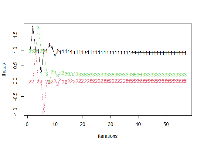
See information about the running Julia environment (e.g., the list
of loaded Julia libraries) with jlme_status():
jlme_status()
#> jlme 0.4.1
#> R version 4.4.1 (2024-06-14 ucrt)
#> Julia Version 1.10.5
#> Commit 6f3fdf7b36 (2024-08-27 14:19 UTC)
#> Build Info:
#>   Official https://julialang.org/ release
#> Platform Info:
#>   OS: Windows (x86_64-w64-mingw32)
#>   CPU: 8 × 11th Gen Intel(R) Core(TM) i7-1165G7 @ 2.80GHz
#>   WORD_SIZE: 64
#>   LIBM: libopenlibm
#>   LLVM: libLLVM-15.0.7 (ORCJIT, tigerlake)
#> Threads: 1 default, 0 interactive, 1 GC (on 8 virtual cores)
#> Status `C:\Users\jchoe\AppData\Local\Temp\jl_NI67vu\Project.toml`
#>   [38e38edf] GLM v1.9.0
#>   [ff71e718] MixedModels v4.27.0
#>   [3eaba693] StatsModels v0.7.4
#>   [9a3f8284] Random
On setup, {jlme} loads GLM, StatsModels, and
MixedModels,
as well as those specified in jlme_setup(add). Other
libraries such as Random (required for
parametricbootstrap()) are loaded on an as-needed
basis.
{JuliaConnectoR}While users will typically not need to interact with
{JuliaConnectoR} directly, it may be useful for extending
{jlme} features with other packages in the Julia modelling
ecosystem. A simple way to do that is to use juliaImport(),
which creates makeshift bindings to any Julia library.
Here’s an example replicating a workflow using Effects.empairs
for post-hoc pairwise comparisons:
# New model: 2 (M/F) by 3 (curse/scold/shout) factorial
jmod2 <- jlmer(
  r2 ~ Gender * btype + (1 | id),
  data = lme4::VerbAgg,
  family = "binomial"
)
jmod2
#> <Julia object of type GeneralizedLinearMixedModel>
#>
#> Generalized Linear Mixed Model fit by maximum likelihood (nAGQ = 1)
#>   r2 ~ 1 + Gender + btype + Gender & btype + (1 | id)
#>   Distribution: Bernoulli{Float64}
#>   Link: LogitLink()
#>
#>    logLik    deviance     AIC       AICc        BIC
#>  -4341.4933  8682.9867  8696.9867  8697.0014  8745.5232
#>
#> Variance components:
#>       Column   VarianceStd.Dev.
#> id (Intercept)  1.52160 1.23353
#>
#>  Number of obs: 7584; levels of grouping factors: 316
#>
#> Fixed-effects parameters:
#> ─────────────────────────────────────────────────────────────────
#>                               Coef.  Std. Error       z  Pr(>|z|)
#> ─────────────────────────────────────────────────────────────────
#> (Intercept)                0.738396   0.0956957    7.72    <1e-13
#> Gender: M                  0.404282   0.201612     2.01    0.0449
#> btype: scold              -1.01214    0.0742669  -13.63    <1e-41
#> btype: shout              -1.77376    0.0782721  -22.66    <1e-99
#> Gender: M & btype: scold   0.130832   0.156315     0.84    0.4026
#> Gender: M & btype: shout  -0.533658   0.168832    -3.16    0.0016
#> ─────────────────────────────────────────────────────────────────library(JuliaConnectoR)
# First call downloads the library (takes a minute)
Effects <- juliaImport("Effects")
# Call `Effects.empairs` using R syntax `Effects$empairs()`
pairwise <- Effects$empairs(jmod2, dof = glance(jmod2)$df.residual)
pairwise
#> <Julia object of type DataFrames.DataFrame>
#> 15×7 DataFrame
#> Row │ Gender btype r2: Y err dof t Pr(>|t|) ⋯
#> │ String String Float64 Float64 Int64 Float64 Float64 ⋯
#> ─────┼──────────────────────────────────────────────────────────────────────────
#> 1 │ F > M curse -0.404282 0.201612 7577 -2.00524 0.0449725 ⋯
#> 2 │ F curse > scold 1.01214 0.13461 7577 7.51901 6.15243e-
#> 3 │ F > M curse > scold 0.477022 0.196994 7577 2.4215 0.0154799
#> 4 │ F curse > shout 1.77376 0.136284 7577 13.0152 2.57693e-
#> 5 │ F > M curse > shout 1.90314 0.202352 7577 9.4051 6.75459e- ⋯
#> 6 │ M > F curse > scold 1.41642 0.201127 7577 7.0424 2.05522e-
#> 7 │ M curse > scold 0.881304 0.247263 7577 3.56424 0.0003671
#> 8 │ M > F curse > shout 2.17805 0.202251 7577 10.769 7.53779e-
#> 9 │ M curse > shout 2.30742 0.251552 7577 9.17273 5.84715e- ⋯
#> 10 │ F > M scold -0.535114 0.196498 7577 -2.72326 0.0064789
#> 11 │ F scold > shout 0.761627 0.135565 7577 5.61817 1.99834e-
#> 12 │ F > M scold > shout 0.891002 0.201868 7577 4.41378 1.02988e-
#> 13 │ M > F scold > shout 1.29674 0.197648 7577 6.56086 5.70179e- ⋯
#> 14 │ M scold > shout 1.42612 0.247866 7577 5.75357 9.07797e-
#> 15 │ F > M shout 0.129376 0.202988 7577 0.637355 0.523913
#> 1 column omittedNote that Julia DataFrame objects such as the one above
can be collected into an R data frame using
as.data.frame(). This lets you, for example, apply p-value
corrections using the familiar p.adjust() function in R,
though the option
to do that exists in Julia as well.
pairwise_df <- as.data.frame(pairwise)
cbind(
  pairwise_df[, 1:2],
  round(pairwise_df[, 3:4], 2),
  pvalue = format.pval(p.adjust(pairwise_df[, 7], "bonferroni"), 1)
)
#>    Gender         btype r2..Y  err pvalue
#> 1   F > M         curse -0.40 0.20  0.675
#> 2       F curse > scold  1.01 0.13  9e-13
#> 3   F > M curse > scold  0.48 0.20  0.232
#> 4       F curse > shout  1.77 0.14 <2e-16
#> 5   F > M curse > shout  1.90 0.20 <2e-16
#> 6   M > F curse > scold  1.42 0.20  3e-11
#> 7       M curse > scold  0.88 0.25  0.006
#> 8   M > F curse > shout  2.18 0.20 <2e-16
#> 9       M curse > shout  2.31 0.25 <2e-16
#> 10  F > M         scold -0.54 0.20  0.097
#> 11      F scold > shout  0.76 0.14  3e-07
#> 12  F > M scold > shout  0.89 0.20  2e-04
#> 13  M > F scold > shout  1.30 0.20  9e-10
#> 14      M scold > shout  1.43 0.25  1e-07
#> 15 F > M shout 0.13 0.20 1.000MixedModels.jl supports various display
formats for mixed-effects models which are available in
{jlme} via the format argument of
print():
# Rendered via {knitr} with chunk option `results="asis"`
print(jmod, format = "markdown")| Est. | SE | z | p | σ_Subject | |
|---|---|---|---|---|---|
| (Intercept) | 251.4051 | 6.6323 | 37.91 | <1e-99 | 23.7805 |
| Days | 10.4673 | 1.5022 | 6.97 | <1e-11 | 5.7168 |
| Residual | 25.5918 |
Be sure to pass integers (vs. doubles) to Julia functions that expect Integer type:
jl_put(1)
#> <Julia object of type Float64>
#> 1.0jl_put(1L)
#> <Julia object of type Int64>
#> 1The Dict (dictionary) data type is common and relevant
for modelling workflows in Julia. {jlme} offers
jl_dict() as an opinionated constructor for that
usecase:
# Note use of `I()` to protect length-1 values as scalar
jl_dict(a = 1:2, b = "three", c = I(4.5))
#> <Julia object of type Dict{Symbol, Any}>
#> Dict{Symbol, Any} with 3 entries:
#>   :a => [1, 2]
#>   :b => ["three"]
#>   :c => 4.5
See ?JuliaConnectoR::`JuliaConnectoR-package` for a
comprehensive list of data type conversion rules.
Using MKL.jl
or AppleAccelerate.jl
may improve model fitting performance (but see the system requirements
first). This should be supplied to the add argument to
jlme_setup(), to ensure that they are loaded first, prior
to other packages.
# Not run
jlme_setup(add = "MKL", restart = TRUE)
jlme_status() # Should now see MKL loaded hereIf the data is large, a sizable overhead will come from transferring
the data from R to Julia. If you are also looking to fit many models to
the same data, you should first filter to keep only the columns you need
and then use jl_data() to send the data to Julia. The Julia
object can then be used in place of an R data frame.
data_r <- mtcars

# Keep only columns you need + convert with `jl_data()`
data_julia <- jl_data(data_r[, c("mpg", "am")])

jlm(mpg ~ am, data_julia)
#> <Julia object of type StatsModels.TableRegressionModel>
#>
#> mpg ~ 1 + am
#>
#> ────────────────────────────────────────────────────────────────────────
#>                 Coef.  Std. Error      z  Pr(>|z|)  Lower 95%  Upper 95%
#> ────────────────────────────────────────────────────────────────────────
#> (Intercept)  17.1474      1.1246   15.25    <1e-51   14.9432     19.3515
#> am            7.24494     1.76442   4.11    <1e-04    3.78674    10.7031
#> ────────────────────────────────────────────────────────────────────────
If your data has custom contrasts, you can use
jl_contrasts() to also convert that to Julia first before
passing it to the model.
data_r$am <- as.factor(data_r$am)
contrasts(data_r$am) <- contr.sum(2)

data_julia <- jl_data(data_r[, c("mpg", "am")])
contrasts_julia <- jl_contrasts(data_r)

jlm(mpg ~ am, data_julia, contrasts = contrasts_julia)
#> <Julia object of type StatsModels.TableRegressionModel>
#>
#> mpg ~ 1 + am
#>
#> ────────────────────────────────────────────────────────────────────────
#>                 Coef.  Std. Error      z  Pr(>|z|)  Lower 95%  Upper 95%
#> ────────────────────────────────────────────────────────────────────────
#> (Intercept)  20.7698     0.882211  23.54    <1e-99   19.0407    22.4989
#> am: 1        -3.62247    0.882211  -4.11    <1e-04   -5.35157   -1.89337
#> ────────────────────────────────────────────────────────────────────────If you spend non-negligible time fitting regression models for your work, please just learn Julia! It’s a great high-level language that feels close to R in syntax and its REPL-based workflow.
The JuliaConnectoR R package for powering the R interface to Julia.
The Julia packages GLM.jl, StatsModels, and MixedModels.jl for interfaces to and implementations of (mixed effects) regression models.
Other R interfaces to MixedModels. It has come to my attention
after working on this for a while and publishing it to CRAN that there
were prior efforts by Mika
Braginsky in {jglmm} and by
Philip Alday in {jlme}. These
packages/scripts predate {JuliaConnectoR} (which I find to
be leaner and more robust) and are instead built on top of {JuliaCall}.
These binaries (installable software) and packages are in development.
They may not be fully stable and should be used with caution. We make no claims about them.