The hardware and bandwidth for this mirror is donated by METANET, the Webhosting and Full Service-Cloud Provider.
If you wish to report a bug, or if you are interested in having us mirror your free-software or open-source project, please feel free to contact us at mirror[@]metanet.ch.

litterfitter

R package for fitting and testing alternative models for single cohort litter decomposition data

Installation

  #install.packages("remotes")
  remotes::install_github("cornwell-lab-unsw/litterfitter")
  
library(litterfitter)

Getting started

At the moment there is one key function which is fit_litter which can fit 6 different types of decomposition trajectories. Note that the fitted object is a litfit object

fit <- fit_litter(time=c(0,1,2,3,4,5,6),
                  mass.remaining =c(1,0.9,1.01,0.4,0.6,0.2,0.01),
                  model="weibull",
                  iters=500)

class(fit)

You can visually compare the fits of different non-linear equations with the plot_multiple_fits function:

plot_multiple_fits(time=c(0,1,2,3,4,5,6),
                   mass.remaining=c(1,0.9,1.01,0.4,0.6,0.2,0.01),
                   model=c("neg.exp","weibull"),
                   iters=500)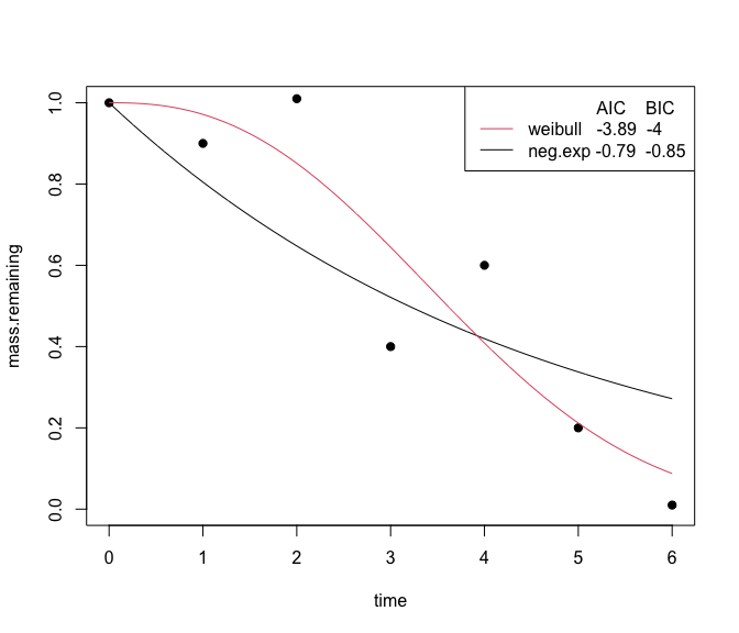

Calling plot on a litfit object will show you the data, the curve fit, and even the equation, with the estimated coefficients:

   plot(fit)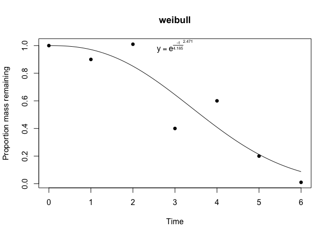

The summary of a litfit object will show you some of the summary statistics for the fit.

#> Summary of litFit object
#> Model type: weibull 
#> Number of observations:  7 
#> Parameter fits: 4.19 
#> Parameter fits: 2.47 
#> Time to 50% mass loss: 3.61 
#> Implied steady state litter mass: 3.71 in units of yearly input 
#> AIC:  -3.8883 
#> AICc:  -0.8883 
#> BIC:  -3.9965

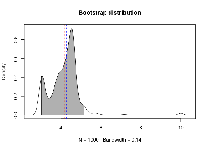
From the litfit object you can then see the uncertainty in the parameter estimate by bootstrapping

These binaries (installable software) and packages are in development.
They may not be fully stable and should be used with caution. We make no claims about them.