The hardware and bandwidth for this mirror is donated by METANET, the Webhosting and Full Service-Cloud Provider.
If you wish to report a bug, or if you are interested in having us mirror your free-software or open-source project, please feel free to contact us at mirror[@]metanet.ch.

Toolkit for Viral Quasispecies Comparison from Long-Read Sequencing performing variety of viral quasispecies diversity analyses based on long-read sequence alignment. Main functions include 1) sequencing error/noise minimization and read sampling, 2) Single nucleotide variant (SNV) profiles comparison, and 3) viral quasispecies profiles comparison and visualization.
‘longreadvqs’ is a package available on CRAN and can be installed
easily in R:
{r, eval=FALSE} install.packages("longreadvqs")
If you have a problem installing QSutils,
a key dependency of this package, please do the following:
{r, message=FALSE, warning=FALSE, results = "hide", eval=FALSE} install.packages("devtools") library(devtools) install_git("https://github.com/VHIRHepatiques/QSutils")
Viral quasispecies (VQS) refers to a genetically closely related population of viral variants. Measurement of VQS diversity, especially in highly mutating RNA viruses, is vital for understanding their micro-evolution. Long-read sequencing facilitates retrieving full-length sequences of specific genes or genomes from each variant, yet challenges like sequencing errors and low coverage depth hinder diversity metric computation and comparison. Here, we present methodologies to overcome these challenges, enabling comparisons of VQS diversity.
Sequencing errors create plenty of artificial single nucleotide variants (SNVs), leading to an overestimated number of singleton haplotypes (haplotype = group of identical reads, singleton haplotype = haplotype with only a single read). Our package aims to minimize potential sequencing errors and potential noises from rare mutations along long reads defined as SNV(s) or nucleotide base(s) with a frequency less than n % at each nucleotide position. Such problematic base(s) will be replaced with the consensus or majority base of that particular position.
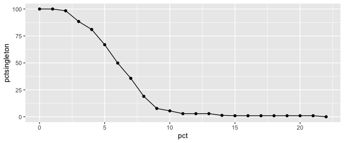
First, load the “longreadvqs” package and a FASTA file of example read alignment (sample1.fasta). To choose the % cut-off for noise minimization, use the “pctopt” function that shows % singleton haplotypes in the read alignment across different % cut-offs. Then, use the “vqssub” function for noise minimization, in this case, we choose a 10% cut-off that decreases singleton haplotypes to less than 10% of all reads. This function will give a summary of VQS diversity metrics calculated by the “QSutils” package (Gregori, et al., 2016) after noise minimization.
library(longreadvqs)

#Load sample 1.
sample1 <- system.file("extdata", "sample1.fasta", package = "longreadvqs")
#Check which % cut-off could effectively minimize noises by assessing % singleton haplotypes.
library(ggplot2)
x <- pctopt(sample1, pctsing = 0, label = "sample1")
ggplot(x, aes(x=pct, y=pctsingleton)) + geom_line() + geom_point()
#VQS diversity metrics of noise minimized (10% cut-off) read alignment
vqssub(sample1, pct = 10, label = "sample1")
#>     label  method samplingwhen pct fulldepth depth haplotypes nsingleton
#> 1 sample1 conbase        after  10       311   311         47         17
#>   pctsingleton polymorph mutations  shannon norm_shannon gini_simpson      FAD
#> 1     5.466238         6       116 2.917347    0.7577235    0.8819625 6.475025
#>           Mfe         Pie         Mfm         Pim
#> 1 0.002580953 0.002994924 6.79165e-09 0.001803544
To compare VQS diversity across samples, it’s important to standardize the read alignment depth. Since sequencing results can vary, we perform down-sampling after minimizing noises with the “vqssub” function. In our case, for sample1, sample2, and sample3 with original depths of 311, 316, and 655, respectively, we randomly down-sample them to a common depth of 300.
#Load samples 2 and 3.
sample2 <- system.file("extdata", "sample2.fasta", package = "longreadvqs")
sample3 <- system.file("extdata", "sample3.fasta", package = "longreadvqs")

#Noise minimization (10% cut-off) and down-sampling (depth of 300)
a <- vqssub(sample1, pct = 10, samsize = 300, label = "sample1")
b <- vqssub(sample2, pct = 10, samsize = 300, label = "sample2")
c <- vqssub(sample3, pct = 10, samsize = 300, label = "sample3")

#Compare VQS diversity across three samples after noise minimization and down-sampling.
rbind(a, b, c)
#>     label  method samplingwhen pct fulldepth depth haplotypes nsingleton
#> 1 sample1 conbase        after  10       311   300         44         16
#> 2 sample2 conbase        after  10       316   300         56         24
#> 3 sample3 conbase        after  10       655   300         28          4
#>   pctsingleton polymorph mutations  shannon norm_shannon gini_simpson      FAD
#> 1     5.333333         6       108 2.875905    0.7599792    0.8799554 5.626911
#> 2     8.000000         7       135 3.126571    0.7767200    0.8977035 9.861366
#> 3     1.333333         5        53 2.670116    0.8013062    0.8943813 1.845056
#>           Mfe         Pie          Mfm         Pim
#> 1 0.002548420 0.002974055 7.016045e-09 0.001782496
#> 2 0.002457405 0.003201742 6.025138e-09 0.001891865
#> 3 0.002147954 0.002440550 5.532911e-09 0.001636262
We can also repeatedly down-sample the alignments and check the consistency of each VQS diversity metric at the different depths like the following example.
#Randomly down-sample from depth of 655 to 300, and 100 (10 iterations for each sample size).
set.seed(123)
c_full <- vqssub(sample3, pct = 10, label = "full_depth") #non-sampled alignment
c_300 <- vqsresub(sample3, iter = 10, pct = 10,
                  samsize = 300, label = "depth_300") #down-sample to depth of 300
c_100 <- vqsresub(sample3, iter = 10, pct = 10,
                  samsize = 100, label = "depth_100") #down-sample to depth of 100

all_c <- rbind(c_full, c_300, c_100) #combine data

#Load packages for visualization.
library(cowplot)

all_c$depth <- as.character(all_c$depth)
depthorder <- c("655", "300", "100")

#Plot box-plots of three VQS metrics variation through different sampling depths.
haplotypes <- ggplot(all_c, aes(x = factor(depth, level=depthorder), y = haplotypes,
    group = interaction(depth, label), fill = label)) + geom_boxplot() +
  xlab("depth") + theme(legend.position = "none")
shannon <- ggplot(all_c, aes(x = factor(depth, level=depthorder), y = shannon,
    group = interaction(depth, label), fill = label)) + geom_boxplot() +
  xlab("depth") + theme(legend.position = "none")
gini_simpson <- ggplot(all_c, aes(x = factor(depth, level=depthorder), y = gini_simpson,
    group = interaction(depth, label), fill = label)) + geom_boxplot() +
xlab("depth") + theme(legend.position = "none")plot_grid(haplotypes, shannon, gini_simpson, nrow = 1)
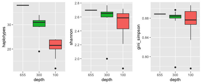
From this plot, the number of haplotypes obviously decreases as the depth decreases, while Shannon entropy and the Gini-Simpson index remain relatively stable with high variation at a depth of 100.
The previous “vqssub” function just summarizes key VQS diversity metrics after noise minimization and down-sampling. However, these metrics do not provide us with comprehensive data for further comparative analyses, such as SNV positions and full read alignment after down-sampling. The “vqsassess” function will generate a complete VQS profile for each sample, and the outputs can be used for other functions.
In this example, we repeat noise minimization and down-sampling for samples 1-3 but apply the “vqsassess” function instead of the “vqssub” function. We then compare the SNV profiles between these samples using the “snvcompare” function.
#Generate complete VQS data for further comparison for each sample.
s1 <- vqsassess(sample1, pct = 10, samsize = 300, label = "sample1")
s2 <- vqsassess(sample2, pct = 10, samsize = 300, label = "sample2")
s3 <- vqsassess(sample3, pct = 10, samsize = 300, label = "sample3")
#Compare SNV profile between three samples.
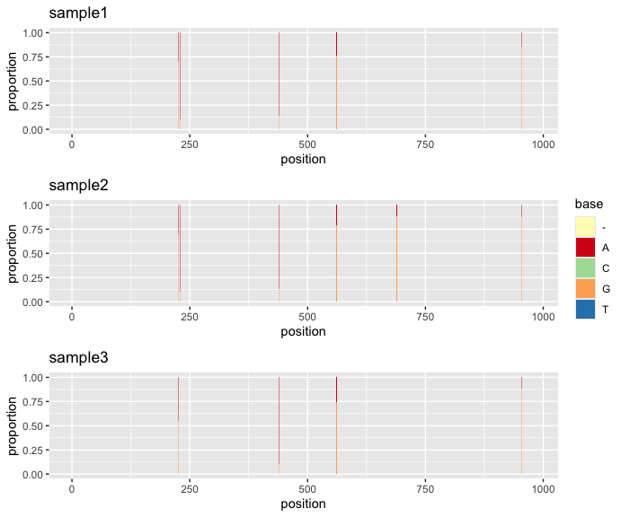
snvcompare(samplelist = list(s1, s2, s3), ncol = 1)
This plot shows that SNV positions are well-aligned between three samples. In some cases, SNV plot can highlight sequencing error concentrating at a particular range in read alignment like the additional sample added to the following example.
#Load sample 4.
sample4 <- system.file("extdata", "mock.fasta", package = "longreadvqs")
s4 <- vqsassess(sample4, pct = 10, samsize = 300, label = "sample4")
#SNV profile of sample 4
s4$snv
The plot above captures atypical SNVs towards the 3’ end of the sample 4 alignment, which is potentially caused by sequencing error. We can address this issue using the “vqscustompct” function, which allows us to adjust the % cut-off for noise minimization at specific range(s) in the alignment. In the case of sample 4, we increase the % cut-off from position 972 onward, raising it from 10% to 30%.
#Use "vqscustompct" function to increase % cut-off after position 972 to 30%.
s4_fix <- vqscustompct(sample4, pct = 10, brkpos = c("1:971","972:982"), lspct = c(10,30),
                       samsize = 300, label = "sample4")
#SNV profile of sample 4 after % cut-off adjustment
s4_fix$snv
Once we have all samples prepared, we can combine them to not only compare within-sample diversity but also explore between-sample relationships. Using the “vqscompare” function, noise-minimized down-sampled reads from all samples are pooled to identify 1) identical haplotypes and 2) genetically closely related haplotypes between samples. In this example, we combine the previously prepared outputs of samples 1 to 4 into the “vqscompare” function, allowing it to generate a summary comparative plot.
#List outputs from "vqsassess" or "vqscustompct" that we want to compare into "vqscompare" function.
#Set the number of new OTU groups based on k-means clustering to 10 groups (kmeans.n = 10).
set.seed(1234)
comp <- vqscompare(samplelist = list(s1, s2, s3, s4_fix),
                   lab_name = "Sample", kmeans.n = 10)
#The most important output of the "vqscompare" function is the summary plot.
comp$summaryplot
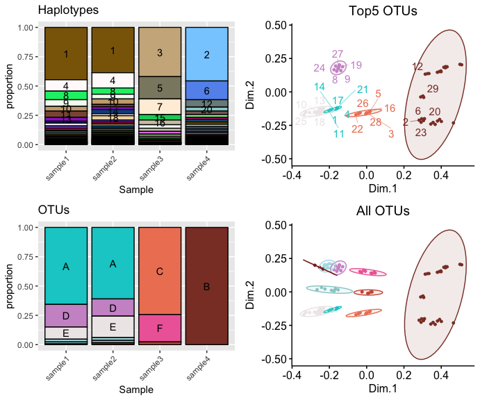
The summary plot comprises four main subplots. First, the haplotype plot at the top left displays all unique haplotypes and their proportions across all samples. Second, the operational taxonomic unit (OTU) plot at the bottom left groups genetically closely related haplotypes into new OTUs through k-means clustering on a multidimensional scale (MDS) of all samples’ pairwise SNV distances. Third, the MDS plot at the top right visualizes the genetic relationships and clustering scheme of the five largest OTUs and haplotypes belonging to each OTU. Fourth, the MDS plot at the bottom right shows all classified OTUs.
In our example, samples 1 to 4 represent read alignments of the influenza A virus (IAV)’s M segment, gathered from patients in the same ward (Williams, et al., 2023). Based on our comparison, patients of samples 1 and 2 likely contracted the same virus, as evidenced by the similarity in both VQS haplotype profiles and OTU profiles. Meanwhile, patients of samples 3 and 4 appear to have been infected with distinct sets of viruses, differing from each other and from those in samples 1 and 2. Despite these distinctions, the MDS plots indicate that the genetic distances between all samples are not significantly far apart. This suggests that these diversities may not be adequately captured at the consensus gene level.
https://doi.org/10.21203/rs.3.rs-4637890/v1
These binaries (installable software) and packages are in development.
They may not be fully stable and should be used with caution. We make no claims about them.