The hardware and bandwidth for this mirror is donated by METANET, the Webhosting and Full Service-Cloud Provider.
If you wish to report a bug, or if you are interested in having us mirror your free-software or open-source project, please feel free to contact us at mirror[@]metanet.ch.

lspline: Linear Splines with Convenient Parametrisations

• Examples
  • Setting knot locations manually
  • Knots at n equal-length intervals
  • Knots at quantiles of x
• Installation
• Acknowledgements

Linear splines with convenient parametrisations such that

• coefficients are slopes of consecutive segments
• coefficients capture slope change at consecutive knots

Knot locations can be specified

• manually (lspline())
• at breaks dividing the range of x into q equal-frequency intervals (qlspline())
• at breaks dividing the range of x into n equal-width intervals (elspline())

Examples

Examples of using lspline(), qlspline(), and elspline(). We will use the following artificial data with knots at x=5 and x=10

set.seed(666)
n <- 200
d <- data.frame(
  x = scales::rescale(rchisq(n, 6), c(0, 20))
)
d$interval <- findInterval(d$x, c(5, 10), rightmost.closed = TRUE) + 1
d$slope <- c(2, -3, 0)[d$interval]
d$intercept <- c(0, 25, -5)[d$interval]
d$y <- with(d, intercept + slope * x + rnorm(n, 0, 1))

Plotting y against x:

library(ggplot2)
fig <- ggplot(d, aes(x=x, y=y)) + 
  geom_point(aes(shape=as.character(slope))) +
  scale_shape_discrete(name="Slope") +
  theme_bw()
fig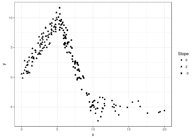

The slopes of the consecutive segments are 2, -3, and 0.

Setting knot locations manually

We can parametrize the spline with slopes of individual segments (default marginal=FALSE):

library(lspline)
m1 <- lm(y ~ lspline(x, c(5, 10)), data=d)
knitr::kable(broom::tidy(m1))

Or parametrize with coeficients measuring change in slope (with marginal=TRUE):

m2 <- lm(y ~ lspline(x, c(5,10), marginal=TRUE), data=d)
knitr::kable(broom::tidy(m2))

The coefficients are

• lspline(x, c(5, 10), marginal = TRUE)1 - the slope of the first segment
• lspline(x, c(5, 10), marginal = TRUE)2 - the change in slope at knot x = 5; it is changing from 2 to -3, so by -5
• lspline(x, c(5, 10), marginal = TRUE)3 - tha change in slope at knot x = 10; it is changing from -3 to 0, so by 3

The two parametrisations (obviously) give identical predicted values:

all.equal( fitted(m1), fitted(m2) )
## [1] TRUE

graphically

fig +
  geom_smooth(method="lm", formula=formula(m1), se=FALSE) +
  geom_vline(xintercept = c(5, 10), linetype=2)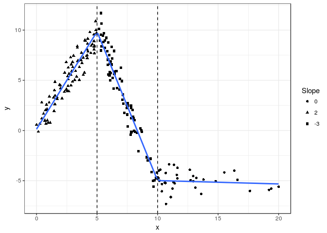

Knots at n equal-length intervals

Function elspline() sets the knots at points dividing the range of x into n equal length intervals.

m3 <- lm(y ~ elspline(x, 3), data=d)
knitr::kable(broom::tidy(m3))

Graphically

fig +
  geom_smooth(aes(group=1), method="lm", formula=formula(m3), se=FALSE, n=200)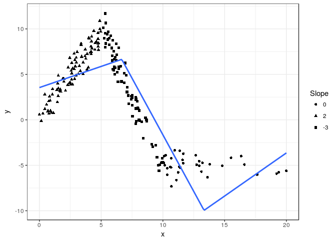

Knots at quantiles of x

Function qlspline() sets the knots at points dividing the range of x into q equal-frequency intervals.

m4 <- lm(y ~ qlspline(x, 4), data=d)
knitr::kable(broom::tidy(m4))

Graphically

fig +
  geom_smooth(method="lm", formula=formula(m4), se=FALSE, n=200)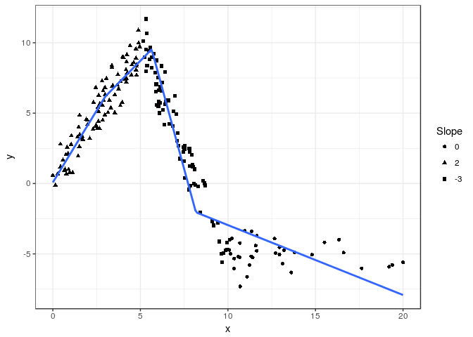

Installation

Stable version from CRAN or development version from GitHub with

devtools::install_github("mbojan/lspline", build_vignettes=TRUE)

Acknowledgements

Inspired by Stata command mkspline and function ares::lspline from Junger & Ponce de Leon (2011). As such, the implementation follows Greene (2003), chapter 7.5.2.

• Greene, William H. (2003) Econometric analysis. Pearson Education
• Junger & Ponce de Leon (2011) ares: Environment air pollution epidemiology: a library for timeseries analysis. R package version 0.7.2 retrieved from CRAN archives.

These binaries (installable software) and packages are in development.
They may not be fully stable and should be used with caution. We make no claims about them.