The hardware and bandwidth for this mirror is donated by METANET, the Webhosting and Full Service-Cloud Provider.
If you wish to report a bug, or if you are interested in having us mirror your free-software or open-source project, please feel free to contact us at mirror[@]metanet.ch.

mcp: Regression with Multiple Change Points

mcp is regression with multiple change points, inferring full Bayesian uncertainty for all parameters, including the change points themselves. At its simplest, it feels like lm() with one formula per segment. At its most flexible, it aims to be brms for change points:

GLMM and distributional regression: Gaussian, binomial, Bernoulli, Poisson, and Negative Binomial families. Group-level (random) effects, AR/MA, and regression on distributional parameters (e.g., sigma, shape).
Express expert knowledge: Specify the number of change points, the form of each segment, and restrict coefficients via priors. Compare hypotheses using loo() and hypothesis().
Native feel: summary(), plot_pars(), pp_check(), and as_draws_df() follow the conventions of brms, rstanarm, and posterior, adapted to change point regression. Inspect the sampled JAGS model in fit$jags_code.

mcp has 200+ academic citations across ecology, astronomy, neuroscience, epidemiology, and other disciplines. You will find many aliases for change point regression in the literature, including piecewise linear, discontinuity, segmented, and broken stick regression.

Install

Install mcp from CRAN:

install.packages("mcp")

or install the development version from GitHub:

if (!requireNamespace("remotes")) install.packages("remotes")
remotes::install_github("lindeloev/mcp@dev")

mcp uses JAGS through rjags. If installation of rjags reports that JAGS headers or libraries are missing, install JAGS 4.x and rerun the mcp installation. JAGS 5 is supported when rjags 5 is released.

At a glance

mcp takes a list of formulas - one for each segment:

library(mcp)

model = list(
  response ~ 1,  # plateau (Intercept_1)
  ~ 0 + time,    # joined slope (time_2) at cp_1
  ~ 1 + time     # disjoined slope (Intercept_3, time_3) at cp_2
)

data = mcp_example_data("demo")
fit = mcp(model, data)

The change points are the values of the change-point variable (here time) where the model switches from one formula to the next. The first formula is just response ~ predictors and the most common formula for segment 2+ would be ~ predictors (more details here).

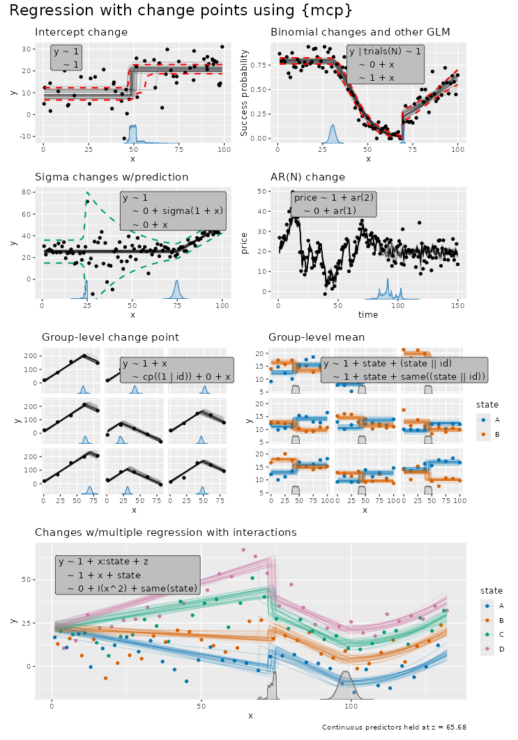
You can do change point regression for a large number of models in a syntax that aligns with lm()/glm()/brms. E.g.:

Brief worked example

The following model infers the two change points between three segments. You can run this complete worked example (which fits the model and plots by default) in one line:

library(mcp)
demo_fit = mcp_example("demo")  # Also check out other examples

See demo_fit$example_code for how it was generated, and explore more demos in mcp_example(). But for now, let’s walk through the example manually:

# Define the model
model = list(
  response ~ 1,  # plateau (Intercept_1)
  ~ 0 + time,    # joined slope (time_2) at cp_1.
  ~ 1 + time     # disjoined slope (Intercept_3, time_3) at cp_2
)

# Get example data and fit it: mcp(model, data, ...)
fit = mcp(model, demo_fit$data, sample = "both")

Plot and summary

The default plot includes data, fitted lines drawn randomly from the posterior, and change point(s) posterior density for each chain. Here we also add the 95% central interval of the fitted values (interval = "fitted"):

plot(fit, interval = "fitted") + ggtitle("Regression with two change points")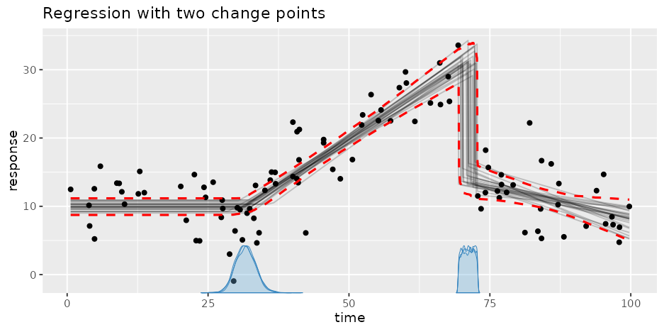

Use summary() to summarise the posterior distribution as well as sampling diagnostics:

summary(fit)

## Family: gaussian
## Links: mu = identity; sigma = identity
## Draws: 9000 (3 chains with iter = 3000)
## Segments:
##   1: response ~ 1
##   2: ~ 0 + time
##   3: ~ 1 + time
## 
## Change point parameters:
##    parameter   mean    sd  lower  upper rhat ess_bulk ess_tail    sim match
##  cp_1        31.7   1.8   28.4   35.3   1.00     3301     4250 30.0      OK
##  cp_2        71.15  0.99  69.47  72.78  1.00     3649     6590 70.00     OK
## 
## Population-level parameters:
##    parameter   mean    sd  lower  upper rhat ess_bulk ess_tail    sim match
##  Intercept_1  9.94  0.66   8.62  11.22  1.00     4835     6307 10.00     OK
##  time_2       0.546 0.047  0.456  0.642 1.00     5165     6622  0.500    OK
##  Intercept_3 14.0   1.3   11.4   16.6   1.00     2306     4675 15.0      OK
##  time_3      -0.206 0.082 -0.366 -0.045 1.00     1287     2440 -0.300    OK
##  sigma_1      3.87  0.28   3.36   4.46  1.00     4455     4623  3.50     OK

rhat is the rank-normalized split-Rhat convergence diagnostic.
ess_bulk and ess_tail are the effective sample sizes for the bulk and tails of the posterior. Warning thresholds can be changed with mcp(..., diagnostics = list(rhat = 1.01, ess_bulk = 400, ess_tail = 400)); summary() inherits these settings.
In this case, we simulated data using mcp (see how in demo_fit$example_code) so the columns sim and match show true value and whether it was recovered.

plot_pars(fit) can be used to inspect the posteriors and convergence of all parameters. See the documentation of plot_pars() for many other plotting options. Here, we plot just the (population-level) change points. They often have “strange” posterior distributions, highlighting the need for a computational approach:

plot_pars(fit, regex_pars = "cp_") + ggtitle("Change point posteriors")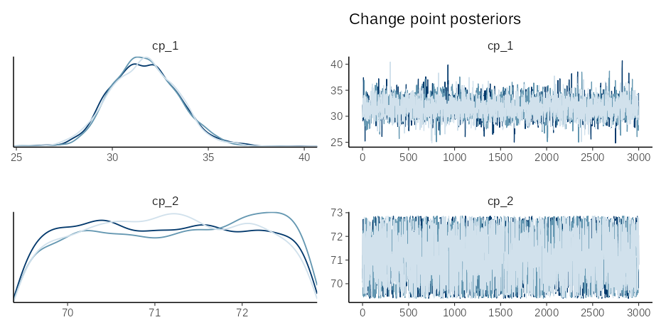

Do a posterior predictive check to see if the model recovers the empirical distribution in the data:

pp_check(fit) + ggtitle("Posterior Predictive check for change point regression")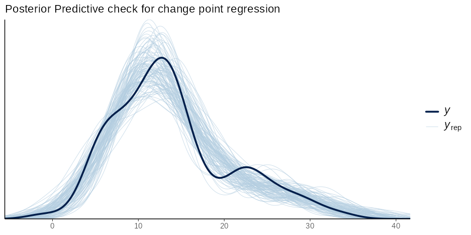

You can expect most generics from R, posterior, tidybayes to work on mcpfits. E.g., use fitted(fit) and predict(fit) to get fits and predictions for in-sample and out-of-sample data, use as_draws(fit) to get draws (see ?as_draws.mcpfit for all formats), etc.

Tests and model comparison

We can test (joint) probabilities in the model using hypothesis() (see more here). For example, what is the evidence (given priors) that the first change point (cp_1) is later than 30 against it being earlier than 30?

hypothesis(fit, "cp_1 > 30")

## # A tibble: 1 × 7
##   hypothesis     mean    sd lower upper  prob    BF
##   <chr>         <dbl> <dbl> <dbl> <dbl> <dbl> <dbl>
## 1 cp_1 - 30 > 0  1.67  1.79 -1.63  5.28 0.826  4.92

For model comparisons, we can fit a null model and compare the predictive performance of the two models using (approximate) leave-one-out cross-validation (see more here). Let’s specify a null model where the first two segments are reduced to one straight line, i.e., removing the change point:

# Define the model
model_null = list(response ~ 1 + time)  # Intercept_1 and time_1

# Fit it
fit_null = mcp(model_null, demo_fit$data)

Leveraging the power of loo::loo(), we see that the two-change-points model is preferred (it is on top), and both p_worse and the elpd_diff / se_diff ratio indicate this preference is strong:

fit_loo = loo(fit)
fit_null_loo = loo(fit_null)

loo::loo_compare(fit_loo, fit_null_loo)

##   model elpd_diff se_diff p_worse diag_diff diag_elpd
##  model1       0.0     0.0      NA                    
##  model2     -58.2     9.0    1.00

Learn more

The articles on the mcp website go in-depth with the functionality of mcp:

Modeling

Understanding mcp formulas: how segments connect (joined ~ 0 + x vs. disjoined ~ 1 + x), parameter names, same(), and the model math.
Group-level (random) effects: group-level intercepts, slopes, and change points, e.g., (1 | id) and cp((1 | id)).
Variance and other distributional parameters: change points in, e.g., the residual SD using sigma(1 + x).
Time series and autocorrelation: ar() and ma() terms, including change points in autocorrelation.

Families

Supported families and link functions: gaussian(), binomial(), bernoulli(), poisson(), and negbinomial().
Poisson and negative binomial and Binomial and Bernoulli: worked examples, including rates via offset().

Inference

Using priors and Default priors: set and check priors, including on change points.
Hypotheses and model comparison: loo(), directional hypothesis() tests, and Savage-Dickey Bayes factors.
Fits and predictions: fitted() and predict(), including forecasting with future change points.
Plotting: plot(), plot_dpar(), plot_pars(), pp_check(), and your own ggplot2 plots.
Missing responses and imputation: change points in gaps of the data and imputations of missing responses.

Implementation

From formulas to sampler code: how mcp writes the JAGS model in fit$jags_code.
Diagnosing and fixing problems: convergence, speed, and common errors.

Citation

This preprint formally introduces mcp. Find citation info at the link, call citation("mcp") or copy-paste this into your reference manager:

  @Article{,
    title = {mcp: An R Package for Regression With Multiple Change Points},
    author = {Jonas Kristoffer Lindeløv},
    journal = {OSF Preprints},
    year = {2020},
    doi = {10.31219/osf.io/fzqxv},
    encoding = {UTF-8},
  }

These binaries (installable software) and packages are in development.
They may not be fully stable and should be used with caution. We make no claims about them.