The hardware and bandwidth for this mirror is donated by METANET, the Webhosting and Full Service-Cloud Provider.
If you wish to report a bug, or if you are interested in having us mirror your free-software or open-source project, please feel free to contact us at mirror[@]metanet.ch.
mcstatsim packageThe mcstatsim package offers an efficient, functional
programming-based approach for statistical simulations, centralizing the
process in a single higher-order function for better
manageability. Besides, it includes ready-to-use functions for
well-known simulation targets.
The core runsim() function processes simulation
parameters via expanded grid, mapping them to the simulation
function.
Outputs are deliberately structured as dataframe to simplify analysis and visualization, addressing the limitations of list outputs in data manipulation.
You can install the latest development version of
mcstatsim from gitHub:
# install.packages("devtools")
#devtools::install_github("ielbadisy/mcstatsim")Here is a basic example to get you started with
mcstatsim:
library(mcstatsim)

# Define a simple simulation function
sim_function <- function(a, b) {
  Sys.sleep(0.5)  # Simulate a time-consuming process
  return(data.frame(result = a + b))
  }

# Generate a grid of parameters
params <- expand.grid(a = 1:3, b = 4:6)

# Run simulations
results <- runsim(n = 3, grid_params = params, sim_func = sim_function, show_progress = TRUE)
This example demonstrates how to define a simple simulation function,
create a grid of parameters for the simulation, and run the simulations
in parallel using mcstatsim.
To illustrate the utility of this package in a concrete example, we
will simulate the evaluation of several imputation methods to assess
their effectiveness in preserving the accuracy of coefficient estimates
in a Cox regression model. This will demonstrate the creation of a
simulation function, setting up parameters, and using
mcstatsim to run these simulations in parallel.
Simulation aim: We will to assess the performance of some imputation methods regarding their capacity to preserve the values of coefficients estimates. For this aim, we well set up the following simulation design:
Generate fully observed data ->
data_complete
estimate the beta coefficients values from
data_complete
Introduce missigness under MCAR to complete dataset generated in
(1) -> data_missing
impute the dataset generated at (3) ->
data_imputed
Use the following simulation targets to compute the distortion
between \(\beta_{true}\) from
data_complete and \(\beta_i\) from
data_imputed:
\[ \text{Bias}(\hat{\beta}) = E[\hat{\beta}] - \beta_{\text{true}} \]
\[ \text{Coverage} = \frac{1}{N} \sum_{i=1}^{N} \mathbf{1}(\beta_{\text{true}} \in \text{CI}_i) \]
\[ \text{MSE} = E[(\hat{\beta} - \beta_{\text{true}})^2] \]
NB: All these metrics (and more) are already implemented in
the mcstatsim package (see ?calc_bias(),
?calc_coverage(), and ?calc_rmse().
Since we want to preserve the spirit of the functional prgramming style, all our simulation design step will be decomposed as helper functions. In others words, the simulation steps will be translated to functions as follow:
pacman::p_load(mcstatsim, survival, dplyr, ggplot2)

## (1) generate fully observed data -> `data_complete`
gencox <- function(n = 300, maxTime = 7, logHR = 0.5) {
  lambda <- 0.1
  rho <- 1.6
  rateC <- 0.09

  # covariates
  x1 <- rnorm(n)
  x2 <- x1^2 + x1 + runif(n)
  x3 <- rbinom(n, 1, 0.5)

  # estimated survival times
  U <- runif(n)
  Tlat <- (-log(U) / (lambda * exp(logHR * (x1 + x2 + x3))))^(1 / rho)
  Ctimes <- rexp(n, rate = rateC)

  # follow-up times and event indicators
  time <- pmin(Tlat, Ctimes)
  status <- as.numeric(Tlat <= Ctimes)
  time <- ifelse(time > maxTime, maxTime, time)
  status <- ifelse(time >= maxTime, 1, status)

  data <- data.frame(time, status, x1, x2, x3)
  data$x3 <- as.factor(data$x3)

  return(data)
  }

## (2) estimate the beta coefficients values from `data_complete`
estimate_coxest <- function(data) {
  myFormula <- survival::Surv(time, status) ~ x1 + x2 + x3
  coefs <- summary(survival::coxph(myFormula, data = data))$coef
  coefs[, 1]
}

## (3) introduce missigness under MCAR to complete dataset generated in (1) -> `data_missing`
introduce_MCAR <- function(x, covariates = names(x), p = 0.3) {

  stopifnot(is.data.frame(x), p >= 0 && p <= 1, all(covariates %in% names(x)))
  x[covariates] <- lapply(x[covariates], function(z) {
    z[sample(length(z), floor(p * length(z)))] <- NA
    z
  })

  return(x)
}

## (4) impute the dataset generated at (3) -> `data_imputed`
imputer <- function(data, method) {
  stopifnot(is.data.frame(data))
  if (is.factor(method)) {method <- as.character(method)}

  supported_methods <- c("knn", "cart", "missforest", "missranger", "misscforest", "complete")
  stopifnot(method %in% supported_methods)

  data_imputed <- switch(method,
                 knn = VIM::kNN(data)[names(data)],
                 cart = simputation::impute_cart(data, .~.),
                 missforest = missForest::missForest(data, xtrue = data, verbose = FALSE)$ximp,
                 missranger = missRanger::missRanger(data, pmm.k = 5, num.trees = 100, verbose = 0),
                 misscforest = suppressWarnings(missCforest::missCforest(data, ntree = 10L)),
                 complete = data[stats::complete.cases(data), ])

  return(data_imputed)
  }

## (5) compute the simulation targets
evaluate_coxest <- function(data, truelogHR) {
  myFormula <- survival::Surv(time, status) ~ x1 + x2 + x3
  coefs <- summary(survival::coxph(myFormula, data = data))$coef
  estimates <- as.data.frame(coefs)

  out <- data.frame(
    estimates = estimates$coef,
    ci_lower = estimates$coef - 1.96 * estimates$`se(coef)`,
    ci_upper = estimates$coef + 1.96 * estimates$`se(coef)`
    )

  out$bias <- mcstatsim::calc_bias(out$estimates, truelogHR)$bias
  out$coverage <- mcstatsim::calc_coverage(out$ci_lower, out$ci_upper, truelogHR)$coverage
  out$rmse <- mcstatsim::calc_rmse(out$estimates, truelogHR)$rmse

  return(out)
}simcox <- function(n, logHR, pmiss, covariates = c("x2"), method = method){
data_complete <- gencox(n = n)
truelogHR <- estimate_coxest(data_complete)
data_missing <- introduce_MCAR(data_complete, covariates = covariates, p = pmiss)
data_imputed <- imputer(data_missing, method = method)
res_est <- evaluate_coxest(data_missing, truelogHR = truelogHR)
res <- cbind(n, pmiss, method, covariates, res_est, row.names = NULL)
return(res)
}Now, to link our simulation function to the simulation parameters, we will generate a grid of paremeters with the same names as the argument of simulation function:
params <- expand.grid(n = c(200, 500),
                      logHR = 0.5,
                      pmiss = c(0.2, 0.5),
                      method = c("knn", "cart", "missforest", "missranger",
"misscforest", "complete"))In one line of code, we can lunch our simulation:
set.seed(123)
sim_res <- runsim(n = 100, grid_params = params, sim_func = simcox, show_progress = FALSE, num_cores = 6)Finaly, we retreive all the results in one single dataset (i.e
sim_res) for ploting and table production:
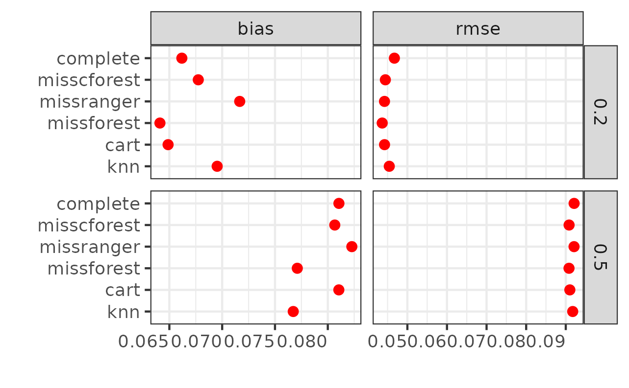
sim_res$bias <- abs(sim_res$bias)

sim_res2 <- gather(sim_res, metric, value, c(bias, rmse))
ggplot(sim_res2, aes(x=value, y=method, fill=method)) +
  stat_summary(fun=mean, geom="point", shape=20, size=3, color="red") +
  theme_bw() +
  theme(axis.text.x = element_text(hjust = 1),
        legend.position = "none") +
  labs(x = "", y = "") +
  facet_grid(pmiss~metric, scales="free")

ggsave("quick_res.png")
Let’s skip interpreting the results since the simulation design isn’t
complete yet—we need to add more simulation targets and assess different
hyperparameter values. However, this provides a good demonstration of
how the mcstatsim package can efficiently organize Monte
Carlo simulations without the complexities of for-loops and managing
numerous parameters.
Functional programming approach: Streamlines the process of setting up and running simulations.
Parallel execution: Leverages parallel computing to speed up the execution of simulations.
Structured output: Returns simulation results in a dataframe, facilitating quick analysis and visualization.
The major improvement in version 0.5.0 compared to version 0.1.0 is
the integration of parallel computing support using the
future package backend within the pbapply
package. This enhancement overcomes the previous limitation, which only
supported multicore parallel computing on Unix-based operating systems
through parallel::mcmapply(). With this update,
mcstatsim now supports parallel computing across various
operating systems, including Windows, thereby providing greater
flexibility and performance improvements for users.
Contributions are welcome! If you’d like to help improve
mcstatsim, please feel free to submit a pull request.
These binaries (installable software) and packages are in development.
They may not be fully stable and should be used with caution. We make no claims about them.