
The hardware and bandwidth for this mirror is donated by METANET, the Webhosting and Full Service-Cloud Provider.
If you wish to report a bug, or if you are interested in having us mirror your free-software or open-source project, please feel free to contact us at mirror[@]metanet.ch.
When unidentified human remains are found, forensic scientists must search databases of missing persons to find potential identifications. mispitools provides a statistical framework based on likelihood ratios (LRs) to quantify the weight of evidence, combining genetic and non-genetic information, and support decision-making in these investigations.
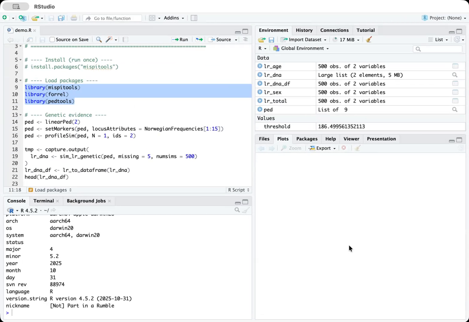
Tutorial by Suisei Nakagawa
The likelihood ratio is the gold standard for evidence evaluation in forensic science. Rather than providing a binary “yes/no” answer, the LR tells us how much the evidence should change our belief about an identification.
We evaluate evidence under two competing hypotheses:
\[LR = \frac{P(\text{Evidence} \mid H_1)}{P(\text{Evidence} \mid H_2)}\]
The LR is not a probability of identification. It measures the relative support provided by the evidence, which can then be combined with prior information to make decisions.
# From CRAN
install.packages("mispitools")

# Development version
devtools::install_github("MarsicoFL/mispitools")Consider a realistic scenario: a family reports a person missing, and investigators need to search a database of unidentified individuals. The family provides a DNA sample from a relative (e.g., a grandparent), and investigators have information about the missing person’s physical characteristics.
We simulate LR distributions from DNA evidence. This requires defining a pedigree structure connecting the MP to the reference individual who provided a DNA sample.
library(mispitools)
library(forrel)
library(pedtools)

# Define pedigree: grandparent-grandchild relationship
ped <- linearPed(2)  # 3-generation pedigree
ped <- setMarkers(ped, locusAttributes = NorwegianFrequencies[1:15])
ped <- profileSim(ped, N = 1, ids = 2)  # Simulate reference profile

# Simulate LRs under both hypotheses
lr_dna <- sim_lr_genetic(ped, missing = 5, numsims = 500)
lr_dna_df <- lr_to_dataframe(lr_dna)

head(lr_dna_df)
#>      Related  Unrelated
#> 1  1247.3201  0.0023415
#> 2   892.1547  0.0001823
#> ...
The Related column contains LRs simulated under H1 (when
the POI truly is the MP), while Unrelated contains LRs
under H2 (when the POI is unrelated).
Physical characteristics such as biological sex, estimated age, and anthropological features also provide evidential value:
# Simulate LR distributions for sex and age
lr_sex <- sim_lr_prelim("sex", numsims = 500)
lr_age <- sim_lr_prelim("age", numsims = 500)

head(lr_sex)
#>    Related Unrelated
#> 1    1.863    0.1052
#> 2    1.863    1.8627
#> ...When evidence sources are conditionally independent, their LRs multiply. This is a fundamental property of the Bayesian framework:
# Combine DNA + sex + age
lr_total <- lr_combine(lr_dna_df, lr_sex)
lr_total <- lr_combine(lr_total, lr_age)

# Visualize the combined LR distribution
plot_lr_distribution(lr_total)
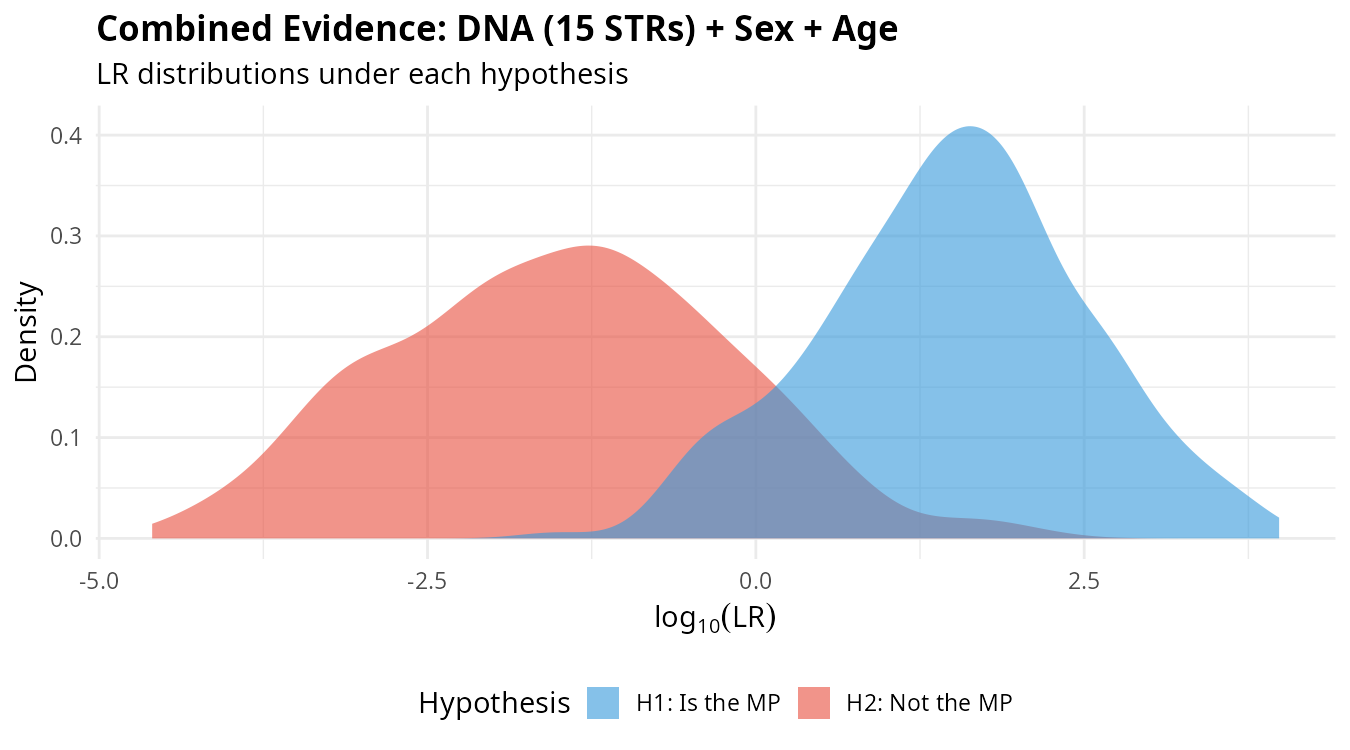
The separation between distributions under H1 (blue) and H2 (red) reflects the discriminating power of the combined evidence. Greater separation means better ability to distinguish between the two hypotheses.
In practice, we search databases containing unidentified individuals. Each candidate receives an LR based on all available evidence, and candidates are ranked accordingly:
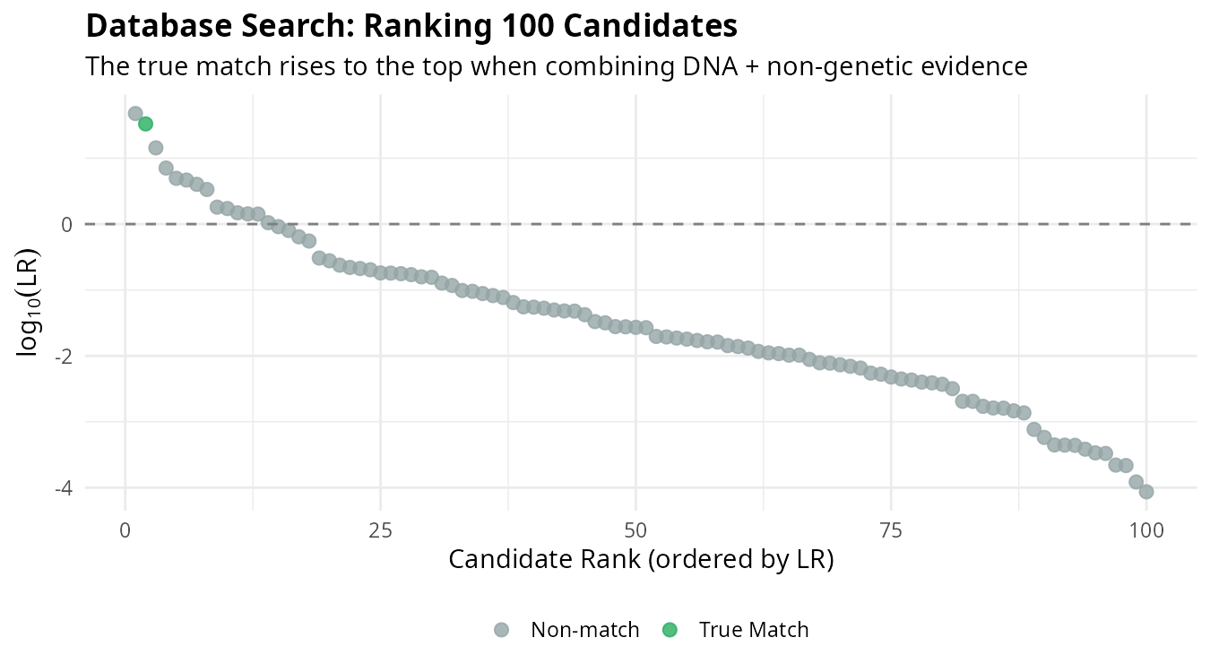
The individual corresponding to the actual MP (blue) rises to the top of the ranking. This demonstrates how combining multiple evidence sources improves our ability to identify the correct individual among many candidates.
To convert LRs into decisions, we analyze error rates at different thresholds:
# Find optimal threshold balancing false positives and false negatives
threshold <- decision_threshold(lr_total, weight = 10)

# Examine error rates at this threshold
threshold_rates(lr_total, threshold)
The weight parameter reflects the relative cost of false
positives versus false negatives. In forensic contexts, falsely
identifying someone (false positive) is typically considered more
serious than failing to identify (false negative).
Two cases with the same combined LR can have very different inferential stability. One may distribute the support evenly across markers; another may owe most of its weight to a single marker — and would collapse if that marker were challenged. mispitools quantifies this with the inclusion concentration index \(C_W^+\) and the leave-one-out diagnostic, and provides a per-case reportable statement:
# Per-marker LRs from forrel::missingPersonLR() or sim_lr_genetic()
lrs_per_marker <- c(D3S1358 = 5.2, TH01 = 12.0, D21S11 = 3.1, FGA = 8.4)

# Calibrate the pedigree-specific cutoff under H_p
cal <- calibrate_concentration_cutoff(
  reference = ped, missing = 5,
  numsims = 1500, probs = 0.90
)

# Per-case fragility report against the calibrated cutoff
fr <- fragility_report(
  per_marker_lrs = lrs_per_marker,
  cutoff = cal$cutoff, probs = cal$probs
)
fr$flag        # TRUE if leave-one-out review is required
fr$statement   # natural-language sentence for the case file
The framework — axiomatic characterization of \(C_W^+\), the leave-one-out identity, and complementarity with population-level mis-specification bounds — is developed in Marsico & Egeland (in preparation).
The combined LR is a single number, but the evidence arrives in pieces. The trajectory of the posterior as each piece is added carries information the endpoint does not: whether belief moved steadily or turned on one step, and whether an intermediate state contradicted the final one.
# Prior over the two hypotheses, then one LR vector per evidence step
tr <- belief_trajectory(
  prior    = c(0.05, 0.95),
  lr_list  = list(c(5.2, 1), c(12.0, 1), c(3.1, 1), c(8.4, 1))
)
round(tr, 5)
#>         [,1]    [,2]
#> [1,] 0.05000 0.95000
#> [2,] 0.21488 0.78512
#> [3,] 0.76658 0.23342
#> [4,] 0.91056 0.08944
#> [5,] 0.98844 0.01156

trajectory_metrics(tr)
#> $kl_from_prior
#> [1] 0.00000000 0.07106659 0.76656675 1.05583811 1.25887080
#>
#> $path_length
#> [1] 0.9384421
#>
#> $concentration
#> [1] 0.7031878
Row 1 is the prior and each subsequent row is the posterior after one
more piece of evidence. trajectory_metrics() summarises the
path: kl_from_prior is how far belief has travelled from
the prior at each step, path_length the total distance
covered, and concentration how much of that movement is
owed to a single step. Here the second step alone accounts for most of
the update.
binary_belief_trajectory() is the two-hypothesis
shortcut that takes per-marker LRs directly and returns the cumulative
log10 LR alongside the posterior.
familias_trajectory() extracts the same metrics from a
Familias::FamiliasPosterior result, so a case already
worked up in Familias can be examined without recomputing it.
The non-genetic LRs depend on error rates that are assigned, not measured. A reported LR is only as defensible as the range of assumptions that leaves it unchanged, so the dependence can be traced explicitly:
lr_sensitivity(evidence_type = "sex", param = "eps",
               range = c(0.01, 0.2), steps = 5)
#>   param_value    LR  log10_LR
#> 1      0.0100 1.980 0.2966652
#> 2      0.0575 1.885 0.2753114
#> 3      0.1050 1.790 0.2528530
#> 4      0.1525 1.695 0.2291697
#> 5      0.2000 1.600 0.2041200
A twentyfold change in the assumed error rate moves the LR from 1.98 to 1.60. The evidence is weak either way, and the conclusion does not hinge on the choice — which is the statement worth making in a report.
Steps 1 to 6 estimate the LR distributions by simulation:
sim_lr_genetic() draws profiles and the distribution
emerges from the sample. Version 2.0 adds a second route to the same
quantities. Given the pedigree and the allele frequencies, the
distribution of the LR is determined, so it can be computed rather than
sampled. There is no simulation error to report and no
numsims to choose; the cost moves elsewhere, to the size of
the pedigree, as described at the end of this section.
The engine is written in C++ and is reached through four entry points.
A marker model bundles a pedigree, a marker, its allele frequencies and a mutation or linkage specification. It validates on construction, so a bad frequency vector fails immediately rather than halfway through a computation.
library(mispitools)
library(pedtools)

freqs <- get_allele_freqs(Argentina)
drop0 <- function(f) { f <- f[f > 0]; f / sum(f) }   # keep alleles present in the marker

ped <- nuclearPed(1)
mk  <- c("THO1", "D3S1358", "VWA")
models <- lapply(mk, function(m)
  marker_model(ped, marker_id = m, freqs = drop0(freqs[[m]]),
               mutation = list(model = "equal", rate = 1e-3)))
names(models) <- mk

models$THO1
#> <marker_model>
#>   marker_id : THO1
#>   alleles   : 10 (4, 5, 6, 7, 8, 9, ...)
#>   mutation  : equal (rate=0.001)
#>   linkage   : none
#>   pedigree  : 3 individuals
Mutation may be "none", "equal",
"stepwise", or the asymmetric model of Dawid (2002). Linked
pairs of markers are handled by Elston-Stewart peeling, with the
recombination fraction stated rather than assumed to be 0.5.
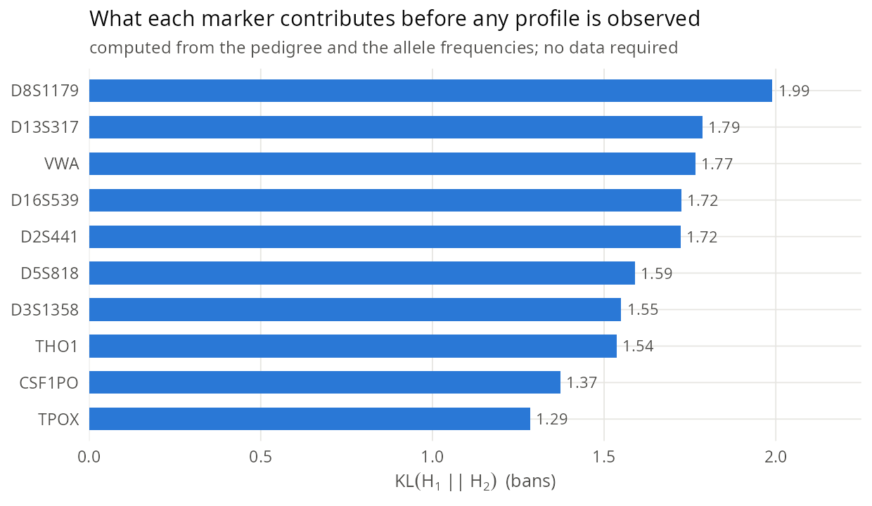
The Kullback-Leibler divergence between the two hypotheses measures the discriminating power of a marker. It depends only on the pedigree and the frequencies, so it can be read before the case has any data, which is useful when deciding which markers to type.
per_marker_kl_profile(models, poi = "3")
#>    marker e_log10_lr_h1 e_log10_lr_h2 kl_h1_to_h2 kl_h2_to_h1
#> 1    THO1     0.6672821     -2.599175    1.536474    5.984822
#> 2 D3S1358     0.6730551     -2.582336    1.549767    5.946048
#> 3     VWA     0.7670269     -2.807222    1.766145    6.463868
e_log10_lr_h1 is the expected weight of evidence when
the POI is the missing person. The two KL columns are asymmetric on
purpose: a marker can be much better at excluding than at including, and
the difference is what those two numbers show.
Read across a marker set, this is a ranking of what each locus is worth for a given pedigree, obtained without typing anyone.
lr_distribution() returns the whole distribution under
both hypotheses, not a point estimate.
d <- lr_distribution(models, poi = "3", method = "grid", grid_points = 512L)

summary(d)
#> Likelihood-ratio distribution summary
#>                   H1        H2
#> E[log10 LR] 2.107364 -7.988733
#> Var         0.514923 15.675662
#> SD          0.717582  3.959250
#> mass        1.000000  1.000000
#>
#> AUC: 0.99621
#> Quantiles of log10 LR | H1:
#>   2.5%    25%    50%    75%  97.5%
#> 1.0076 1.6488 2.0152 2.4732 3.8472
#> Quantiles of log10 LR | H2:
#>     2.5%      25%      50%      75%    97.5%
#> -16.2133  -9.9845  -8.6104  -5.4044  -1.1908

quantile(d, c(0.05, 0.5, 0.95))
#>       5%      50%      95%
#> 1.190806 2.015211 3.389218
The AUC and the quantiles come from the distribution itself, so they
carry no Monte Carlo error. A statement such as “under H1, five per cent
of cases fall below a log10 LR of 1.19” is exact for this
pedigree and this frequency database.
method = "exact" performs a sparse convolution and
reproduces the convolution atom by atom; method = "grid"
projects onto a lattice, which preserves the total mass and the mean
exactly and discretises only the shape. The choice matters in practice:
composing two markers of 10 and 12 alleles exactly already yields around
2.2 million support points, and that number multiplies with each marker
added. For anything beyond two markers, use the grid.
Non-genetic features enter through the same machinery, each with its
population distribution and its error rate, so they end up on the same
log10 LR scale as the markers instead of being described in
words alongside the genetic result.
nongenetic_feature(type = "sex", observed = "F",
                   db_or_freqs = c(F = 0.5, M = 0.5), error = 0.05)
#> <nongenetic_feature>
#>   type          : sex (categorical)
#>   observed      : F
#>   categories    : 2 (F, M)
#>   reference     : marginal
#> error : eps=0.05Two quantities that a simulation of the usual size does not deliver.
The first is the value of the pedigree itself.
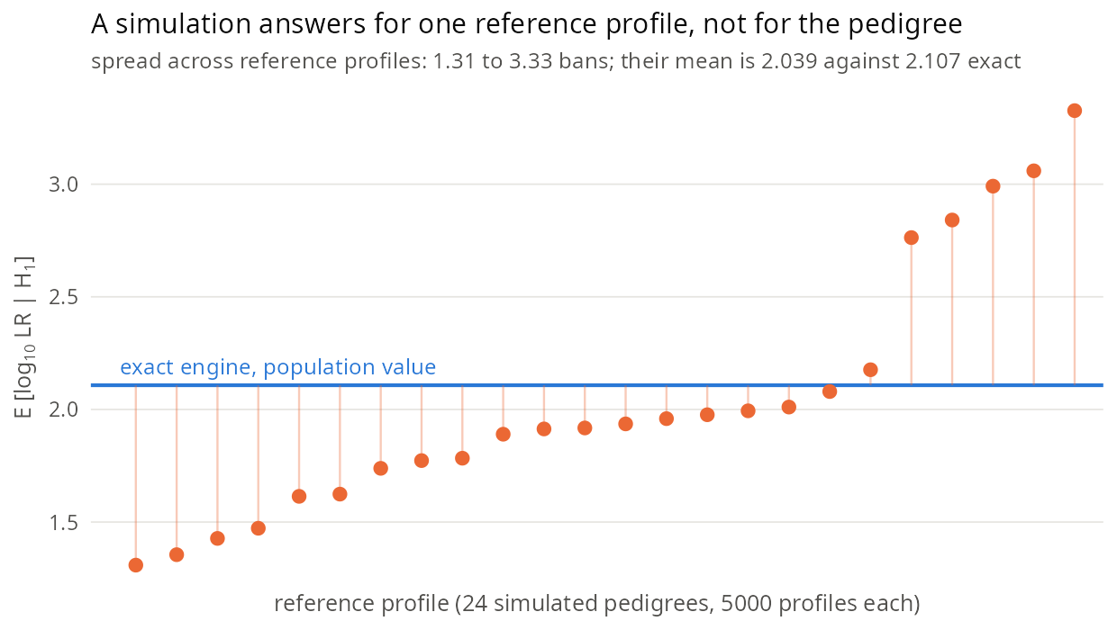
sim_lr_genetic() starts from a reference profile, so the
distribution it returns belongs to that case. Across 24 reference
profiles drawn from the same trio and the same frequency database, the
expected weight of evidence under H1 ranged from 1.31 to 3.33 bans, with
a standard deviation of 0.56. Averaged over them it is 2.04 against the
exact 2.107, a difference of 0.6 standard errors. The two numbers answer
different questions: the simulation says what to expect in the case at
hand, the engine says what the pedigree is worth before any reference
has been typed.
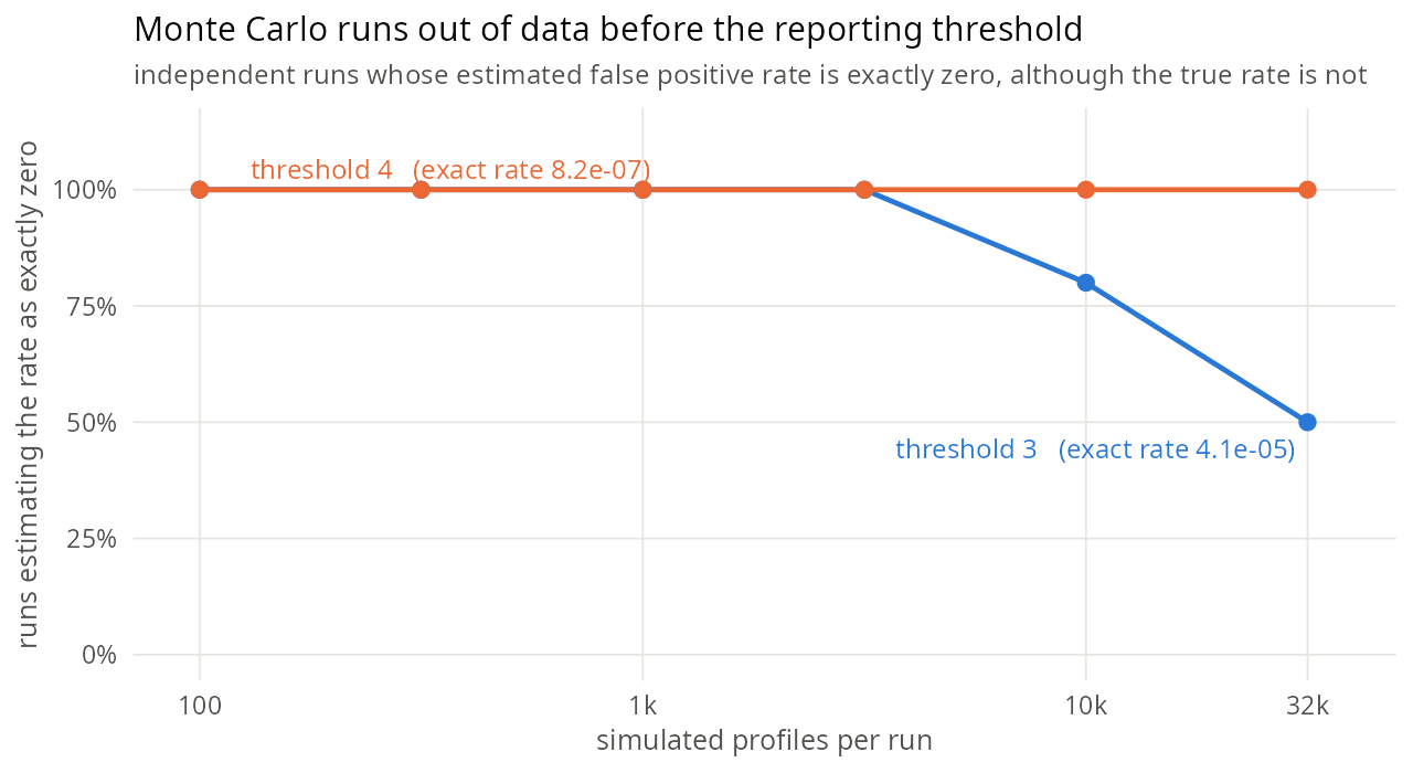
The second is the tail. The false positive rate at the threshold where an identification would be reported is computed directly from the distribution:
threshold log10 LR |
P(log10 LR > t | H2) |
|---|---|
| 2 | 2.11e-03 |
| 3 | 4.09e-05 |
| 4 | 8.16e-07 |
| 5 | 1.31e-08 |
| 6 | 1.85e-10 |
Estimating the same rates by simulation requires observing the events. At threshold 4 the expected number of profiles needed to see a single one is around 1.2 million, and useful precision needs orders of magnitude more. In runs of 1000 profiles the estimate is exactly zero at that threshold; at 32000 profiles, half of the runs still return zero at threshold 3. The estimate is not imprecise there, it is empty.
For the three markers above, the exact distribution takes about one second, while a single simulated run of 32000 profiles takes about five minutes.
The engine enumerates joint genotype states, so its cost is driven by
the number of individuals in the pedigree and by the number of alleles
per marker. On a trio, a marker with 10 to 12 alleles takes about a
second. On a five-individual pedigree such as linearPed(2),
the same computation exceeded 6 GB of memory in our tests. The exact
route is therefore the right tool for trios and small pedigrees; for
larger pedigrees and full profiles, the simulation workflow of Steps 1
to 6 remains the practical one, and the two give answers on the same
scale.
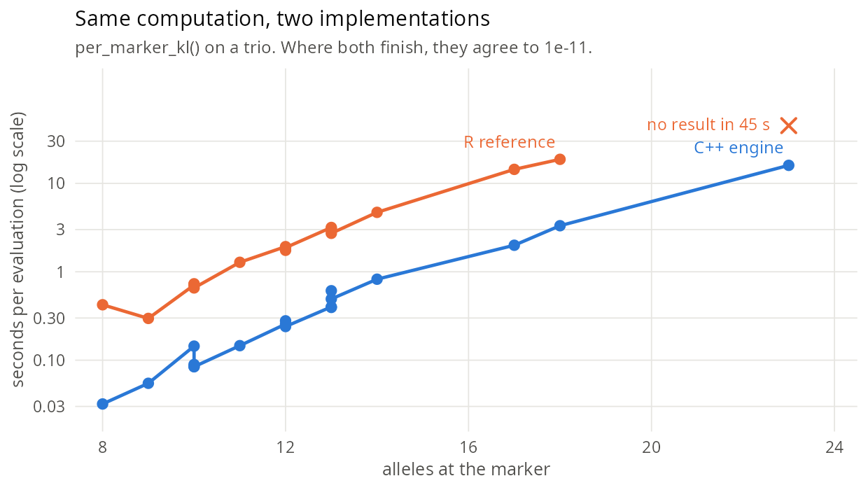
Within that scope the cost is dominated by the number of alleles. The package keeps a reference implementation in R, used as the oracle for the C++ kernel and cross-checked against it in the test suite, so the two can be timed against each other on the same call. On a trio they agree to 1e-11 wherever both finish, and the C++ engine is around seven times faster; at 23 alleles the R implementation returns nothing within 45 seconds while the engine finishes in 16.
For users who prefer a graphical interface, mispitools includes an interactive Shiny application:
mispitools_app()The app is also available online at: https://francomarsico.shinyapps.io/mispitools/
It provides tools for calculating LRs from non-genetic evidence, visualizing probability tables, and exploring decision thresholds.
Version 2.0.0 exports 45 functions. They fall into eight groups.
Simulating evidence. The 1.x route to LR distributions: draw profiles or preliminary data and let the distribution emerge from the sample.
| Function | Purpose |
|---|---|
sim_lr_genetic() |
LR distributions from DNA evidence under H1 and H2, given a pedigree |
sim_lr_prelim() |
LR distributions from non-genetic evidence |
sim_mp_prelim() |
Simulate preliminary investigation data for missing persons |
sim_poi_prelim() |
Simulate preliminary investigation data for persons of interest |
sim_reference_pop() |
Simulate a reference population with pigmentation traits |
Non-genetic likelihood ratios. One LR per feature, each built from a population distribution, an observed value and an error rate.
| Function | Purpose |
|---|---|
lr_sex() |
LR for biological sex |
lr_age() |
LR for age |
lr_birthdate() |
LR for birth date, open or closed search |
lr_hair_color() |
LR for hair colour |
lr_pigmentation() |
LR distributions for joint pigmentation traits (hair, skin, eye) |
lr_compute_pigmentation() |
LRs from conditioned and reference proportions |
error_matrix_hair() |
Hair-colour confusion matrix used as the error model |
cpt_population() |
Population-based conditional probability table |
cpt_missing_person() |
Missing-person-based conditional probability table |
plot_cpt() |
Compare the two conditional probability tables visually |
compute_reference_prop() |
Reference population proportions for pigmentation traits |
compute_conditioned_prop() |
Proportions conditioned on the missing person’s traits |
Combining and reporting.
| Function | Purpose |
|---|---|
lr_combine() |
Combine independent evidence sources |
lr_to_dataframe() |
Convert genetic LR results to a data frame |
plot_lr_distribution() |
Visualise LR distributions under both hypotheses |
Decision analysis. Turning an LR into a decision requires a threshold and an explicit statement of what each kind of error costs.
| Function | Purpose |
|---|---|
decision_threshold() |
Optimal threshold for a given relative cost of errors |
threshold_rates() |
False positive, false negative and related rates at a threshold |
plot_decision_curve() |
Error rates across the range of thresholds |
Fragility and concentration. Two cases with the same combined LR can differ in how evenly the support is spread across markers.
| Function | Purpose |
|---|---|
concentration_index_positive() |
Inclusion concentration index \(C_W^+\) |
concentration_index() |
Concentration of per-step evidence contributions |
herfindahl_index() |
Herfindahl-Hirschman concentration of contributions |
shannon_concentration() |
Entropy-based concentration of contributions |
leave_one_out() |
Per-marker leave-one-out fragility table |
calibrate_concentration_cutoff() |
Pedigree-specific \(C_W^+\) cutoff under \(H_p\) |
fragility_report() |
Per-case reportable fragility statement |
Sequential evidence. How belief moves as the evidence accumulates, not only where it ends.
| Function | Purpose |
|---|---|
belief_trajectory() |
Bayesian belief trajectory over n hypotheses |
binary_belief_trajectory() |
Two-hypothesis trajectory from per-marker LRs |
trajectory_metrics() |
Path length, divergence from prior, concentration |
familias_trajectory() |
The same metrics from a Familias::FamiliasPosterior
result |
entropy_log10() |
Shannon entropy in bans |
kl_divergence_log10() |
Kullback-Leibler divergence in bans |
Exact engine (new in 2.0). The same quantities computed from the pedigree and the allele frequencies rather than sampled.
| Function | Purpose |
|---|---|
marker_model() |
Marker model: pedigree, frequencies, mutation, linkage |
nongenetic_feature() |
Non-genetic evidence on the same log10 LR scale |
get_allele_freqs() |
Population database in the format the engine expects |
lr_distribution() |
Exact distribution of the profile LR under both hypotheses |
per_marker_kl() |
Discriminating power of one marker, before any profile is seen |
per_marker_kl_profile() |
The same across a profile |
as_lr_dist() |
Coerce simulated LRs into the lr_dist class |
The lr_dist object returned by
lr_distribution() has summary(),
quantile(), plot() and print()
methods.
Sensitivity and interface.
| Function | Purpose |
|---|---|
lr_sensitivity() |
Trace an LR across a range of an assumed parameter |
mispitools_app() |
Interactive Shiny application |
The 1.x names remain exported and continue to work, now as deprecated
aliases that emit a message pointing to the current name. Existing
scripts do not break. Among them: simLRgen(),
simLRprelim(), simRef(),
makeMPprelim(), makePOIprelim(),
LRsex(), LRage(), LRdate(),
LRcol(), LRcolors(), combLR(),
CPT_POP(), CPT_MP(), Cmodel(),
LRdist(), deplot(), CondPlot(),
DeT(), Trates(), getfreqs() and
mispiApp(). See ?"mispitools-deprecated" for
the full list of 28.
Marsico FL, Caridi I (2023). “Incorporating non-genetic evidence in large scale missing person searches: A general approach beyond filtering.” Forensic Science International: Genetics, 66, 102891. https://doi.org/10.1016/j.fsigen.2023.102891
Marsico FL, Vigeland MD, et al. (2021). “Making decisions in missing person identification cases with low statistical power.” Forensic Science International: Genetics, 52, 102519. https://doi.org/10.1016/j.fsigen.2021.102519
Egeland T, Marsico FL (2026). “Using all available information in missing person identification.” International Journal of Legal Medicine. https://doi.org/10.1007/s00414-026-03773-6
Franco L. Marsico — Creator and Head Maintainer
Main contributors: - Suisei Nakagawa 
GPL-3
These binaries (installable software) and packages are in development.
They may not be fully stable and should be used with caution. We make no claims about them.

